Versteeg H., Malalasekra W. An Introduction to Computational Fluid Dynamics: The Finite Volume Method

Подождите немного. Документ загружается.

12.15 THE SIMPLE CHEMICAL REACTING SYSTEM 367

T (12.86)

where (MW )

is the molecular weight of species k and R

is the universal gas

constant (8.314 kJ/kmol.K).

The ﬂow ﬁeld is in turn affected by changes in temperature and density,

so in addition to the species and enthalpy equations we must solve all the

ﬂow equations. The resultant set of transport equations can be very large.

Models that consider many intermediate reactions require vast computing

resources, so simple models that incorporate only a few reactions are often

preferred in CFD-based combustion procedures. The simplest known pro-

cedure is the simple chemical reacting system (SCRS; see Spalding, 1979),

which is described below in some detail. Other approaches of modelling

turbulent combustion, such as the eddy break-up model and the laminar

ﬂamelet model, are discussed later.

If we are concerned with the global nature of the combustion process

and with ﬁnal major species concentrations only, the detailed kinetics is

unimportant and a global one-step, inﬁnitely fast, chemical reaction can be

assumed where oxidant combines with fuel in stoichiometric proportions to

form products:

1 kg of fuel + s kg of oxidant → (1 + s) kg of products (12.87)

For methane combustion the equation becomes

+ 2O

→ CO

+ 2H

1 mol of CH

2 mol of O

1 mol of CO

2 mol of H

1 kg of CH

+ kg of O

→ 1 + kg of products

The stoichiometric oxygen/fuel ratio by mass s is equal to 64/16 = 4 for

methane combustion. However, equation (12.87) also shows that the rate of

consumption of fuel during stoichiometric combustion is 1/s times the rate

of consumption of oxygen, i.e.

= M

In the SCRS inﬁnitely fast chemical reactions are assumed and the inter-

mediate reactions are ignored. The transport equations for fuel and oxygen

mass fraction are written as

+ div(

u) = div(Γ

grad Y

) + M

(12.88)

+ div(

u) = div(Γ

grad Y

) + M

(12.89)

where Γ

and Γ

∂

(

)

∂

(

)

∂

(MW )

all species

∑

The simple

chemical reacting

system (SCRS)

12.15

ANIN_C12.qxd 29/12/2006 04:44PM Page 367

368 CHAPTER 12 CFD MODELLING OF COMBUSTION

The oxidant stream will have nitrogen which remains unaffected during

simple combustion; the mass fraction of inert species (Y

) remains the same

before and after combustion. Local values of Y

are determined by mixing

only, since the inert species does not take part in combustion (unless forma-

tion of NO is considered). Since the mass fraction of products Y

= 1 − (Y

+ Y

) it is unnecessary to solve a separate equation for Y

It is possible to reduce the number of transport equations even further by

introducing a variable deﬁned as follows:

= sY

− Y

(12.90)

Application of the single diffusion coefﬁcient assumption, Γ

=Γ

D =Γ

allows us to subtract equation (12.89) from s times equation (12.88) and com-

bine the result into a single transport equation for

+ div(

ρφ

u) = div(Γ

grad

) + (sM

− M

) (12.91)

From the one-step reaction assumption (12.87), we have M

= (1/s)M

giving (sM

− M

) = 0, and equation (12.91) reduces to

+ div(

ρφ

u) = div(Γ

grad

) (12.92)

Hence,

is a passive scalar; it obeys the scalar transport equation without

source terms. A non-dimensional variable

called the mixture fraction

may be deﬁned in terms of

as follows:

= (12.93)

where sufﬁx 0 denotes the oxidant stream and 1 denotes the fuel stream. The

local value of

equals 0 if the mixture at a point contains only oxidant and

equals 1 if it contains only fuel.

Equation (12.93) may be written in expanded form as

= (12.94)

If the fuel stream has fuel only we have

]

= 1[Y

]

= 0 (12.95)

and if the oxidant stream contains no fuel we have

]

= 0[Y

]

= 1 (12.96)

In such conditions equation (12.94) may be simpliﬁed as follows:

== (12.97)

In a stoichiometric mixture neither fuel nor oxygen is present in the prod-

ucts, and the stoichiometric mixture fraction

may be deﬁned as

− Y

+ Y

ox,0

fu,1

+ Y

ox,0

[sY

− Y

] − [−Y

]

[sY

]

− [−Y

]

[sY

− Y

] − [sY

− Y

]

[sY

− Y

]

− [sY

− Y

]

−

∂

(

ρφ

)

∂

(

ρφ

)

∂

ANIN_C12.qxd 29/12/2006 04:44PM Page 368

12.15 THE SIMPLE CHEMICAL REACTING SYSTEM 369

= (12.98)

Fast chemistry implies that, at a certain location with a lean mixture, there

is an excess of oxidant and no fuel is present in the products. Hence Y

= 0

if Y

> 0, so

then

= (12.99)

Conversely, in a rich mixture there is a local excess of fuel in the mixture

and there is no oxidant in the products. Hence Y

= 0 if Y

> 0, so

then

= (12.100)

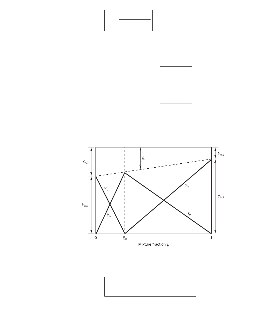
The above formulae show that the mass fractions of the fuel Y

and oxygen

are linearly related to the mixture fraction

. This is illustrated graph-

ically in Figure 12.2.

+ Y

ox,0

fu,1

+ Y

ox,0

−Y

+ Y

ox,0

fu,1

+ Y

ox,0

fu,1

+ Y

ox,0

Figure 12.2 Mixing and

fast reaction between fuel

and oxidant streams

(SCRC relationships)

By equation (12.93)

is linearly related to

so the mixture fraction is

also a passive scalar and obeys the transport equation

+ div(

ρξ

u) = div(Γ

grad

) (12.101)

Written in sufﬁx notation the transport equation for the mixture fraction is

(

ρξ

) + (

) =Γ

(12.102)

To obtain the distribution of

we solve equation (12.101) subject to suitable

boundary conditions, e.g. mixture fractions of fuel and oxidant inlet streams

are known, zero normal ﬂux of

across solid walls and zero-gradient out-

ﬂow conditions. Given the resulting mixture fraction we can rearrange

∂ξ

∂

(

ρξ

)

∂

ANIN_C12.qxd 29/12/2006 04:44PM Page 369

370 CHAPTER 12 CFD MODELLING OF COMBUSTION

equations (12.98)–(12.100) to give values for oxygen and fuel mass fractions

after combustion:

≤

< 1: Y

= 0 Y

= Y

fu,1

(12.103)

0 <

: Y

= 0 Y

= Y

ox,0

(12.104)

The reactants may be accompanied by inert species such as N

, which do not

take part in the reaction. The mass fraction of inert species in the mixture

varies linearly with

, as illustrated in Figure 12.2. Simple geometry gives the

total mass fraction of the inert species Y

after combustion at any value of

= Y

in,0

(1 −

) + Y

in,1

(12.105)

The mass fraction of products (Y

) of combustion may be obtained from

= 1 − (Y

+ Y

) (12.106)

The above equations, (12.101) and (12.103)–(12.106), represent the SCRS

model.

When the reaction products contain two or more species, the ratio of the

mass fraction of each component to the total product mass fraction is known

from the equation for the chemical reaction and can be used to deduce the

mass fraction of different product components. For example, consider the

burning of methane with O

+ 2O

⎯→ CO

+ 2H

1 mol of CH

2 mol of O

1 mol of CO

2 mol of H

16 kg 64 kg 44 kg 36 kg

Ratio of CO

in products by mass (r

) = 44/80

Ratio of H

O in products by mass (r

) = 36/80

If the product mass fraction from equation (12.106) is Y

then the CO

mass

fraction in the products is Y

and the H

O mass fraction is Y

The SCRS model has made the following simpliﬁcations: (i) single-step

reaction between fuel and oxidant, and (ii) one reactant which is locally in

excess causes all the other reactant to be consumed stoichiometrically to

form reaction products. These assumptions ﬁx algebraic relationships between

the mixture fraction

and all the mass fractions Y

, Y

and Y

. As a

consequence of the additional assumption that the mass diffusion coefﬁcients

of all species are equal, it is only necessary to solve one partial differential

equation for

to calculate combusting ﬂows rather than individual partial

differential equations for the mass fraction of each species. An example which

uses this approach for combustion calculations is presented below.

The SCRS model can be readily applied to calculate temperatures and

species distribution in laminar diffusion ﬂames. For example, consider the

axisymmetric laminar non-premixed diffusion ﬂame geometry shown in

−

1 −

Modelling of a

laminar diffusion

flame --- an example

12.16

ANIN_C12.qxd 29/12/2006 04:44PM Page 370

12.16 MODELLING OF A LAMINAR DIFFUSION FLAME 371

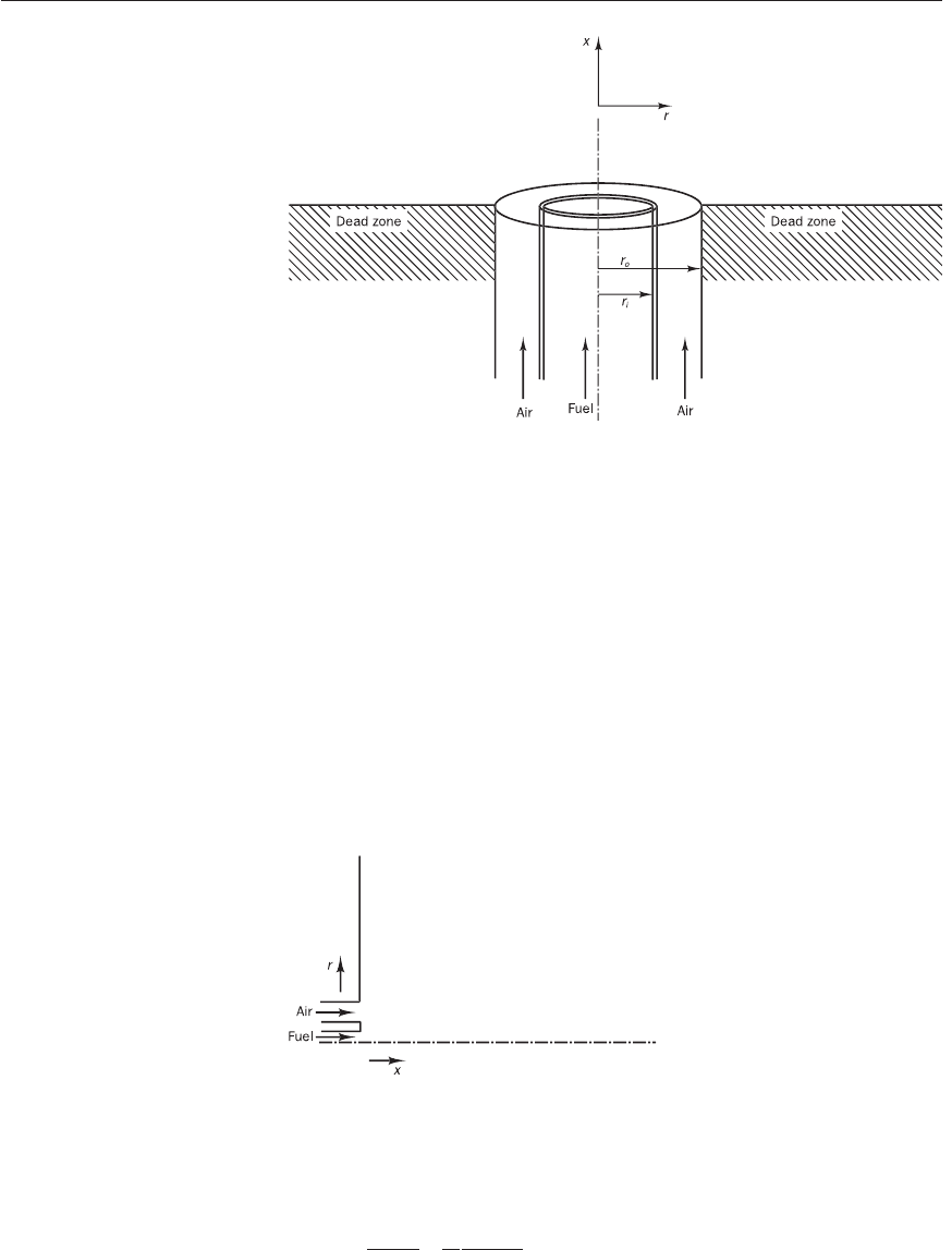
Figure 12.3 Schematic of the

problem considered

Figure 12.4 A part of the

computational geometry

Figure 12.3. The geometry considered here is an experimental conﬁguration

which has been used by a number of studies documented in the combustion

literature (Bennett and Smooke, 1998; Smooke et al., 1990; Smooke, 1991).

For illustrative purposes we use our own operating conditions to formulate

the problem in this example. The radius of the fuel jet (r

) is 0.2 cm and the

radius (r

) of the co-ﬂowing air jet is 2.5 cm. The thickness of the wall

between fuel and air streams is 0.05 cm. Let us consider burning of a pure

methane jet with co-ﬂowing air. Both fuel and air velocities are taken as

0.2 m/s (20 cm/s) and enter at a temperature of 25°C (298 K). We would

like to calculate the resulting ﬂame temperature and major species distribu-

tion ﬁeld for this ﬂame.

For calculation convenience we turn the actual geometry shown in Fig-

ure 12.3 through 90°. The axisymmetry of the problem allows us to adopt

a cylindrical x,r coordinate system to formulate the problem as shown in

Figure 12.4. Here we use u to represent the velocity component in the (axial)

x-direction and v to represent the velocity component in the (radial) r-direction.

The governing equations for steady laminar ﬂow in cylindrical coordinates

in expanded form are as follows (see section 2.3 and section 12.14 above).

Continuity

+=0 (12.107)

∂

(

rv)

∂

(

∂

ANIN_C12.qxd 29/12/2006 04:44PM Page 371

Momentum equations

u-momentum equation:

(

ruu) + (

ruv) = (r

) + (r

) − r (12.108)

v-momentum equation

(

ruv) + (

rvv) = (r

) + (r

) − r (12.109)

The shear stress terms are

2 − (div u) (12.110)

2 − (div u) (12.111)

2 + (12.112)

div u =+ (rv) (12.113)

The momentum equations can be rearranged in the usual form as follows:

u-momentum equation:

(

ruu) + (

ruv) = r

+ r

− r + S

(12.114)

v-momentum equation:

(

ruv) + (

rvv) = r

+ r

− r + S

(12.115)

where S

and S

contain the additional terms arising from the shear stress terms.

Enthalpy equation

uh) + (r

vh) = rD

+ rD

+ S

rad

(12.116)

where D

is the diffusion coefﬁcient for enthalpy (i.e. D

≡

= k/

) and

rad

is the radiation source (or sink) term.

Combustion model

Here we use the SCRC model described in section 12.15. The assumption of

fast chemistry gives the stoichiometric equation

+ 2(O

+ 3.76N

) ⎯→ CO

+ 2H

O + 2 × 3.76N

(12.117)

∂

372 CHAPTER 12 CFD MODELLING OF COMBUSTION

ANIN_C12.qxd 29/12/2006 04:44PM Page 372

12.16 MODELLING OF A LAMINAR DIFFUSION FLAME 373

The stoichiometric oxygen/fuel ratio by mass is

s = 2 × (MW )

/(MW )

= 2 × 32/16 = 4

The mass fraction of fuel in the fuel stream is

fu,1

= 1.0

The mass fraction of oxygen in the air stream is

ox,0

= 0.233 (see section 12.5)

The mass fraction of inert (N

) in the air stream is

in,0

= 0.767

We solve the following equation for the mixture fraction:

) + (r

) = rΓ

+ rΓ

(12.118)

The mass fractions for the fuel and oxidant streams are as follows.

Since the fuel stream has fuel only we have

]

= 1[Y

]

= 0 (12.119)

The oxidant stream contains no fuel but oxygen and nitrogen (inert), so

we have

]

= 0[Y

]

= 0.233 [Y

]

= 0.767 (12.120)

The stoichiometric mixture fraction from equation (12.98) is

==0.055 (12.121)

If heat loss by radiation is considered in the calculation then solution of

the enthalpy equation is required. If radiation is considered to be negligible

then it can be seen that from equation (12.116) when S

rad

= 0 the transport

equation for enthalpy becomes another conserved scalar equation like the

mixture fraction equation. Therefore the enthalpy and mixture fraction are

both scalars and linearly related. The relationship can be further illustrated

as below.

Taking the reference temperature as zero, enthalpy is deﬁned as

h = Y

∆h

fuel

+ c

T (12.122)

Enthalpy of the fuel stream where

= 1 is

fu,in

= Y

fu,in

×∆h

fuel

+ Y

× T

fu,in

where ∆h

fuel

is the enthalpy or formation of fuel. Enthalpy of the air stream

where

= 0 is

air,in

= c

× T

air,in

If we deﬁne a non-dimensional enthalpy as

h* = (12.123)

we can see that when

= 0, Y

= 0, h* = 0 and when

= 1, Y

= 1, h* = 1. If

we make the usual simplifying assumptions – single diffusion coefﬁcient, unity

h − h

air,in

fu,in

− h

air,in

0.233

4 × 1 + 0.233

∂ξ

∂

∂ξ

∂

ANIN_C12.qxd 29/12/2006 04:44PM Page 373

Lewis number, negligible pressure work and radiation source – for enthalpy

transport, the governing transport equations for the enthalpy and mixture

fraction are the same (both variables are passive scalars). The resulting spatial

distributions of non-dimensional enthalpy h* and mixture fraction will be

the same (it is easy to verify that the boundary conditions for both variables

are also identical in this problem). Therefore, we do not need to solve a sep-

arate transport equation for enthalpy, but can calculate this variable from

= h* = (12.124)

Once the enthalpy value and mass fraction of fuel Y

are known from SCRC

relationships, the temperature is obtained from

T = (12.125)

The boundary conditions for the problem are: at the inlet, u

= 0.2 m/s

for both fuel and air streams;

= 1.0 for the fuel stream; and

air

= 0.0

for the air stream. Zero-velocity and zero-mixture-fraction-gradient wall

boundary conditions are used at all solid walls and a constant pressure

boundary condition is imposed on open boundaries with pressure set to

ambient. At the symmetry axis all gradients are set to zero.

Solution of the ﬂuid ﬂow equations and the mixture fraction equation

gives the distribution of mixture fraction which deﬁnes the ﬂame structure

and species distribution. Equations (12.103) and (12.104) are used to obtain

species mass fractions. Equations (12.124) and (12.125) give the enthalpy and

temperature ﬁelds. Using pressure and temperature the density ﬁeld is

obtained from (12.86). Because of the coupled nature of the equations, the

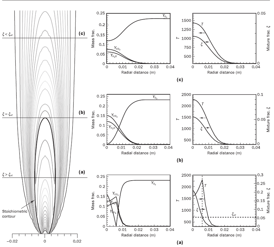
entire solution process is iterative. Figure 12.5 shows some typical results

obtained from this simulation. To highlight the consequences of the fast

chemistry assumption of the SCRS model we show radial proﬁles of tem-

perature and species mass fraction at three different points along the axis as

well as the temperature contours in Figure 12.5. The stoichiometric contour

corresponds with the contour of maximum temperature and deﬁnes the

ﬂame. In the region inside the stoichiometric contour

, so by condition

(12.103) fuel exists here without oxidant. On the other hand, outside the

stoichiometric contour

, so by (12.104) no fuel can exist. At the axial

location (a) where

the radial proﬁles show no oxygen near the axis, and

fuel which gets completely consumed at the

contour. At axial location (b)

where centreline

neither fuel nor oxygen is present and the tempera-

ture is at a maximum. At axial location (c) where centreline

no fuel

exists and the temperature is lower.

Calculations with finite rate chemistry

To include ﬁnite rate and detailed chemistry in this combustion calculation

one has to consider a detailed mechanism and solve many species transport

equations of the form

) + (r

) = r

+ r

+ rM

(12.126)

where M

is the rate of generation of species k, which is determined from

chemical kinetic expressions such as (12.69)–(12.71). Numerical solutions

∂

h − Y

(∆h

)

h − h

air,in

fu,in

− h

air,in

374 CHAPTER 12 CFD MODELLING OF COMBUSTION

ANIN_C12.qxd 29/12/2006 04:44PM Page 374

12.16 MODELLING OF A LAMINAR DIFFUSION FLAME 375

including detailed and ﬁnite rate chemistry result in some variations to the

curves shown in Figure 12.5. The main difference is an overlap of fuel and

oxygen proﬁles and small curvature around the stoichiometric mixture frac-

tion showing a corresponding drop in temperature: see Warnatz et al. (2001).

Comprehensive combustion calculations for this geometry (for different

operating conditions) including detailed chemistry can be found in Smooke

et al. (1990), Bennett and Smooke (1998), Smooke and Bennett (2001).

The method presented above illustrates how CFD can be used for laminar

non-premixed combustion calculations. Unfortunately, the fast chemistry

assumption does not give adequate details of minor species, since it is neces-

sary to include more detailed chemistry and ﬁnite rate kinetics for a more

comprehensive account of combustion. Prediction of pollutants, such as

discussed later in this chapter, inevitably requires inclusion of transport

equations for the most important minor species.

Figure 12.5 Calculated ﬂame structure of a laminar diffusion ﬂame

ANIN_C12.qxd 29/12/2006 04:44PM Page 375

The CFD calculation of turbulent non-premixed combustion is not as

straightforward as laminar calculations, even with the fast chemistry assump-

tion. In Chapter 3 we showed that Reynolds averaging and modelling of

the resulting averages of ﬂuctuating product terms made it possible to

predict incompressible turbulent ﬂow ﬁelds. Equations governing turbulent

non-premixed combustion also require averaging and modelling. The ﬁrst

problem that needs to be addressed is the fact that strong and highly localised

heat generation in combusting ﬂows causes the density to vary as a function

of position in combusting ﬂows. There will also be density ﬂuctuations if the

ﬂow is turbulent. The Reynolds decomposition of a general ﬂow variable is

as follows:

= 2 +

′

For the variables in a reacting ﬂow this yields

= R

+ u′

p = Q + p ′

= 4 +

′

h = P + h′

T = E + T ′

= F

+ Y′

It is easy to demonstrate that the presence of density ﬂuctuations gives

rise to additional terms when Reynolds averaging is used. For example,

consider the instantaneous continuity equation in sufﬁx notation:

+=0 (12.127)

After substituting for u and

the Reynolds-averaged equation is

++ =0 (12.128)

Compare this with the Reynolds-averaged equation for a constant density

ﬂow:

+ (

) = 0 (12.129)

The additional term

∂

()/

∂

in equation (12.128) arises from correla-

tions between the velocity and density ﬂuctuations in a reacting ﬂow and

has to be modelled. Many more terms of this type appear in the Reynolds-

averaged momentum, scalar and species transport equations.

To reduce the number of separate terms requiring modelling in reacting

ﬂows with variable density, we use a density-weighted averaging procedure

known as Favre averaging (Favre, 1969; Jones and Whitelaw, 1982).

In Favre averaging the density-weighted mean velocity is deﬁned as

follows:

U = (12.130)

′u′

∂

∂ρ

∂

(

′u′

)

∂

(4R

)

∂

(

)

∂

∂ρ

∂

376 CHAPTER 12 CFD MODELLING OF COMBUSTION

CFD calculation

of turbulent non-

premixed combustion

12.17

ANIN_C12.qxd 29/12/2006 04:44PM Page 376