Alligood K., Sauer T., Yorke J.A. Chaos: An Introduction to Dynamical Systems

Подождите немного. Документ загружается.

7.6 LYAP U N OV F UNCTIONS

The stability analysis illustrated above for the pendulum relies on Theorem

7.23, due to the Russian mathematician Alexander Mikhailovich Lyapunov.

Theorem 7.23 Let

v be an equilibrium of ˙v ⫽ f(v). If there exists a Lyapunov

function for

v, then v is stable. If there exists a strict Lyapunov function for v, then v

is asymptotically stable.

We refer the reader to (Hirsch and Smale, 1974) for a proof of the theorem.

Note that the energy function of Exercise T7.12 is not a strict Lyapunov function.

It cannot be, since the equilibria are not attracting.

We can now return to the one-dimensional Example 7.20:

x ⫽⫺x

. Linear

analysis is inconclusive in determining the stability of the equilibrium x ⫽ 0. The

next exercise implies that x ⫽ 0 is asymptotically stable.

✎ E XERCISE T7.13

Show that E(x) ⫽ x

is a strict Lyapunov function for the equilibrium x ⫽ 0

x ⫽⫺x

✎ E XERCISE T7.14

Let

x ⫽⫺x

⫹ xy

y ⫽⫺y

⫺ x

. (7.44)

Prove that (0,0) is an asymptotically stable equilibium of (7.44).

Figure 7.17(b) depicts bounded level curves of a strict Lyapunov function for

an equilibrium

v. Since E is strictly decreasing (as a function of t) along solutions,

the solutions (shown with arrows) cut through the level curves of E and converge

v. The sets W

⫽ 兵v 僆 W : E(v) ⱕ c其 can help us understand the extent of the

set of initial conditions whose trajectories converge to an asymptotically stable

equilibrium.

Deﬁnition 7.24 Let

v be an asymptotically stable equilibrium of ˙v ⫽

f(v). Then the basin of attraction of

v, denoted B(v), is the set of initial condi-

tions v

such that lim

t→

⬁

F(t, v

) ⫽ v.

307

D IFFERENTIAL E QUATIONS

Note that any set W on which V is a strict Lyapunov function for v (as in

Deﬁnition 7.22) will be a subset of the basin B(

v).

✎ E XERCISE T7.15

Show that the basin of attraction of the equilibrium (0, 0) for the system

(7.44) is ⺢

A somewhat weaker notion of containment than a basin is that of a “trap-

ping region”—a set in ⺢

where solutions, once they enter, cannot leave as time

increases.

Deﬁnition 7.25 AsetU 傺⺢

is called a forward invariant set for (7.29)

if for each v

僆 U, the forward orbit 兵F(t, v

):t ⱖ 0其 is contained in U. A forward

invariant set that is bounded is called a trapping region. We also require that a

trapping region be an n-dimensional set.

✎ E XERCISE T7.16

Let E be a Lyapunov function on W,letc be a positive real number, and let

⫽ 兵v 僆 W : E(v) ⱕ c其.

(a) Show that, for each c, W

is a forward invariant set. (b) Show that if in

addition E(v) →

⬁

as |v| →

⬁

,thenW

is a trapping region.

Returning to the pendulum example, we reconsider the system under the

effects of a damping force, such as air resistance. Once the pendulum is set into

motion, it will lose energy and eventually come to rest. We assume that the

damping force is proportional to, but opposite in direction from, the velocity of

the pendulum, so that the motion of the pendulum is governed by the equation

x ⫹ b

x ⫹ sin x ⫽ 0, (7.45)

for a constant b ⬎ 0.

From our observations, we would like to be able to conclude that what

were stable equilibria for the undamped pendulum are now asymptotically stable

and attract nearby initial conditions. The fact these equilibria are asymptotically

stable follows from evaluating the Jacobian (check this); however, we are not

able to conclude from the local analysis that all trajectories converge to an

equilibrium. Understanding the technique of Lyapunov functions for conservative

308

7.7 LOTKA-VOLTERRA M ODELS

systems, such as the undamped pendulum, enabled us to draw the phase plane

for this system and view it globally. In that case we were able to understand

the motions for all initial conditions. Unfortunately, total energy is not a strict

Lyapunov function for any equilibria of the damped system. Instead, we compute

E(v) ⫽⫺by

, so that the inequality

E(v) ⬍ 0 fails to be strict for points arbitrarily

near the equilibrium.

Notice that trajectories (other than equilibrium points) do not stay on

the x-axis, the set on which

E ⫽ 0. Therefore we might expect trajectories to

behave as if E were a strict Lyapunov function. The following corollary, often

called “LaSalle’s Corollary” to the Lyapunov Theorem 7.23, not only provides

another means of deducing asymptotic stability for equilibria of the damped

system, but also gives information as to the extent of the basin of attraction for

each asymptotically stable equilibrium. We postpone the proof of the theorem

until Chapter 8 when we study limit sets of trajectories.

Corollary 7.26 (Barbashin-LaSalle) Let E be a Lyapunov function for

on the neighborhood W, as in Deﬁnition 7.22. Let Q ⫽ 兵v 僆 W :

E(v) ⫽ 0其.

Assume that W is forward invariant. If the only forward-invariant set contained

completely in Q is

v, then v is asymptotically stable. Furthermore, W is contained

in the basin of

v; that is, for each v

僆 W, lim

t→

⬁

(F(t, v

)) ⫽ v.

✎ E XERCISE T7.17

Let

x ⫹ b

x ⫹ sin x ⫽ 0, for a constant b ⬎ 0. (a) Convert the differential

equation to a ﬁrst-order system. (b) Use Corollary 7.26 to show that the

equilibria (n

␲

, 0), for even integers n are asymptotically stable. (c) Sketch

the phase plane for the associated ﬁrst-order system.

7.7 LOTKA-VOLTERRA MODELS

A family of models called the Lotka-Volterra equations are often used to simulate

interactions between two or more populations. Interactions are of two types.

Competition refers to the possibility that an increase in one population is bad for

the other populations: an example would be competition for food or habitat. On

the other hand, sometimes an increase in one population is good for the other.

Owls are happy when the mouse population increases. We will consider two cases

of Lotka-Volterra equations, called competing species models and predator-prey

models.

309

D IFFERENTIAL E QUATIONS

We begin with two competing species. Because of the ﬁniteness of resources,

the reproduction rate per individual is adversely affected by high levels of its own

species and the other species with which it is in competition. Denoting the two

populations by x and y, the reproduction rate per individual is

⫽ a(1 ⫺ x) ⫺ by, (7.46)

where the carrying capacity of population x is chosen to be 1 (say, by adjusting

our units). A similar equation holds for the second population y,sothatwehave

the competing species system of ordinary differential equations

x ⫽ ax(1 ⫺ x) ⫺ bxy

y ⫽ cy(1 ⫺ y) ⫺ dxy (7.47)

where a, b, c, and d are positive constants. The ﬁrst equation says the population

of species x grows according to a logistic law in the absence of species y (i.e.,

when y ⫽ 0). In addition, the rate of growth of x is negatively proportional to xy,

representing competition between members of x and members of y. The larger

the population y, the smaller the growth rate of x. The second equation similarly

describes the rate of growth for population y.

The method of nullclines is a technique for determining the global behavior

of solutions of competing species models. This method provides an effective means

of ﬁnding trapping regions for some differential equations. In a competition model,

if a species population x is above a certain level, the fact of limited resources will

cause x to decrease. The nullcline, a line or curve where

x ⫽ 0, marks the boundary

between increase and decrease in x. The same characteristic is true of the second

species y, and it has its own curve where

y ⫽ 0. The next two examples show that

the relative orientation of the x and y nullclines determines which of the species

survives.

E XAMPLE 7.27

(Species extinction) Set the parameters of (7.47) to be a ⫽ 1, b ⫽ 2, c ⫽ 1,

and d ⫽ 3. To construct a phase plane for (7.47), we will determine four regions

in the ﬁrst quadrant: sets for which (I)

x ⬎ 0and

y ⬎ 0; (II)

x ⬎ 0and

y ⬍ 0;

(III)

x ⬍ 0and

y ⬎ 0; and (IV)

x ⬍ 0and

y ⬍ 0. Other assumptions on a, b, c,

and d lead to different outcomes, but can be analyzed similarly.

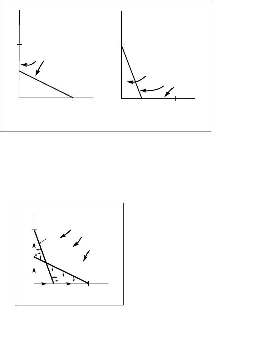
In Figure 7.18(a) we show the line along which

x ⫽ 0, dividing the plane

into two regions: points where

x ⬎ 0 and points where

x ⬍ 0. Analogously,

Figure 7.18(b) shows regions where

y ⬎ 0and

y ⬍ 0, respectively. Combining

the information from these two ﬁgures, we indicate regions (I)–(IV) (as described

above) in Figure 7.19(a). Along the nullclines (lines on which either

x ⫽ 0or

310

7.7 LOTKA-VOLTERRA M ODELS

x = 0

x < 0

x > 0

y < 0

y > 0

y = 0

(a) (b)

Figure 7.18 Method of nullclines for competing species.

The straight line in (a) shows where

x ⫽ 0, and in (b) it shows where

y ⫽ 0for

a ⫽ 1, b ⫽ 2, c ⫽ 1, and d ⫽ 3 in (7.47). The y-axis in (a) is also an x-nullcline,

and the x-axis in (b) is a y-nullcline.

III

Figure 7.19 Competing species: Nullclines.

The vectors show the direction that trajectories move. The nullclines are the lines

along which either

x ⫽ 0or

y ⫽ 0. In this ﬁgure, the x-axis, the y-axis, and the two

crossed lines are nullclines. Triangular regions II and III are trapping regions.

311

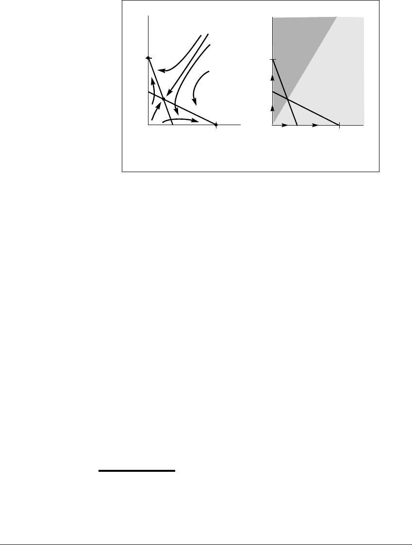
D IFFERENTIAL E QUATIONS

(a) (b)

Figure 7.20 Competing species, extinction.

(a) The phase plane shows attracting equilibria at (1, 0) and (0, 1), and a third,

unstable equilibrium at which the species coexist. (b) The basin of (0, 1) is shaded,

while the basin of (1, 0) is the unshaded region. One or the other species will die

out.

y ⫽ 0), arrows indicate the direction of the ﬂow: left/right where

y ⫽ 0 or up/down

where

x ⫽ 0. Notice that points where the two different types of nullclines cross

are equilibria. There are four of these points. The equilibrium (0, 0) is a repellor;

(1 5, 2 5) is a saddle; and (1, 0) and (0, 1) are attractors.

The entire phase plane is sketched in Figure 7.20(a). Almost all orbits

starting in regions (I) and (IV) move into regions (II) and (III). (The only

exceptions are the orbits that come in tangent to the stable eigenspace of the

saddle (1 5, 2 5). These one-dimensional curves form the “stable manifold” of

the saddle and are discussed more fully in Chapter 10.) Once orbits enter regions

(II) and (III), they never leave. Within these trapping regions, orbits follow the

direction indicated by the derivative toward one or the other asymptotically stable

equilibrium. The basins of attraction of the two possibilities are shown in Figure

7.20(b). The stable manifold of the saddle forms the boundary between the basin

shaded gray and the unshaded basin. We conclude that for almost every choice

of initial populations, one or the other species eventually dies out.

E XAMPLE 7.28

(Coexistence) Set the parameters to be a ⫽ 3, b ⫽ 2, c ⫽ 4, and d ⫽ 3.

The nullclines are shown in Figure 7.21(a). In this case there is a steady state at

(x, y) ⫽ (2 3, 1 2) which is attracting. The basin of this steady state includes

312

7.7 LOTKA-VOLTERRA M ODELS

(a) (b)

Figure 7.21 Competing species, coexistence.

(a) The phase plane shows an attracting equilibrium in which both species survive.

The x-nullcline y ⫽

⫺

x has smaller x-intercept than the y-nullcline y ⫽ 1 ⫺

According to Exercise T7.18, the equilibrium (

) is asymptotically stable. (b) All

initial conditions with x ⬎ 0andy ⬎ 0 are in the basin of this equilibrium.

the entire ﬁrst quadrant, as shown in Figure 7.21(b). Every set of nonzero starting

populations moves toward this equilibrium of coexisting populations.

✎ E XERCISE T7.18

Consider the general competing species equation (7.47) with positive pa-

rameters a, b, c, d. (a) Show that there is an equilibrium with both popu-

lations positive if and only if either (i) both a b and c d are greater than

one, or (ii) both a b and c d are less than one. (b) Show that a positive

equilibrium in (a) is asymptotically stable if and only if the x-intercept of the

x-nullcline is less than the x-intercept of the y-nullcline.

E XAMPLE 7.29

(Predator-Prey) We examine a different interaction between species in this

example in which one population is prey to the other. A simple model of this

interaction is given by the following equations:

x ⫽ ax ⫺ bxy

y ⫽⫺cy ⫹ dxy (7.48)

where a, b, c,andd are positive constants.

313

D IFFERENTIAL E QUATIONS

✎ E XERCISE T7.19

Explain the contribution of each term, positive or negative, to the predator-

prey model (7.48).

System (7.48) has two equilibria, (0, 0) and (

). There are also nullclines;

namely,

x ⫽ 0whenx ⫽ 0orwheny ⫽

, and

y ⫽ 0wheny ⫽ 0orwhenx ⫽

Figure 7.22(a) shows these nullclines together with an indication of the ﬂow

directions in the phase plane.

Unlike previous examples, there are no trapping regions. Solutions appear

to cycle about the nontrivial equilibrium (

). Do they spiral in, spiral out, or

are they periodic? First, check the eigenvalues of the Jacobian at (

✎ E XERCISE T7.20

Find the Jacobian Df for (7.48). Verify that the eigenvalues of Df(

)are

pure imaginary.

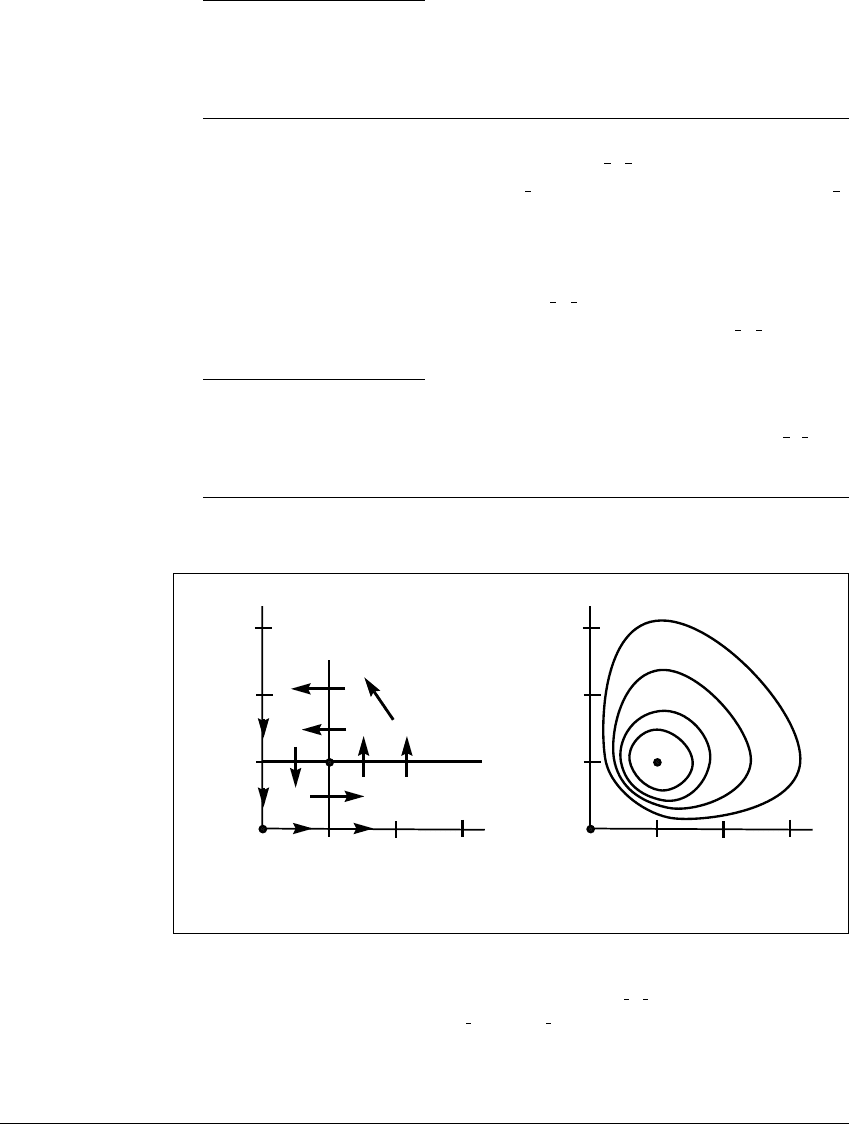
a/b

c/d

a/b

c/d

(a) (b)

Figure 7.22 Predator-prey vector ﬁeld and phase plane.

(a) The vector ﬁeld shows equilibria at (0, 0) and (

). Nullclines are the x-axis,

the y-axis, and the lines x ⫽

and y ⫽

. There are no trapping regions. (b) The

curves shown are level sets of the Lyapunov function E.Since

E ⫽ 0, solutions

starting on a level set must stay on that set. The solutions travel periodically around

the level sets in the counterclockwise direction.

314

7.7 LOTKA-VOLTERRA M ODELS

Since the system is nonlinear and the eigenvalues are pure imaginary, we can

conclude nothing about the stability of (

). Fortunately, we have a Lyapunov

function.

✎ E XERCISE T7.21

Let

E(x, y) ⫽ dx ⫺ c ln x ⫹ by ⫺ a ln y ⫹ K,

where a, b, c, and d are the parameters in (7.48) and K is a constant. Ver-

ify that

E ⫽ 0 along solutions and that E is a Lyapunov function for the

equilibrium (

We can conclude that (

) is stable. Solutions of (7.48) lie on level

curves of E. Since (

) is a relative minimum, these level curves are closed

curves encircling the equilibrium. See Figure 7.22(b). Therefore, solutions of this

predator-prey system are periodic for initial conditions near (

). In fact, every

initial condition with x and y both positive lies on a periodic orbit.

315

D IFFERENTIAL E QUATIONS

☞ C HALLENGE 7

A Limit Cycle in the Van der Pol System

HE LIMITING BEHAVIOR we have seen in this chapter has consisted largely

of equilibrium states. However, it is common for solutions of nonlinear equations

to approach periodic behavior, converging to attracting periodic orbits, or limit

cycles. The Van der Pol equation

x ⫹ (x

⫺ 1)

x ⫹ x ⫽ 0 (7.49)

is a model of a nonlinear electrical circuit that has a limit cycle.

Deﬁning y ⫽

x, the second-order equation is transformed to

x ⫽ y

y ⫽⫺x ⫹ (1 ⫺ x

)y. (7.50)

The origin (0, 0) is the only equilibrium of (7.50), and it is unstable. In this

Challenge, you will show that all other trajectories of the system approach a

single attracting periodic orbit that encircles the origin. This type of limiting

behavior for orbits is a phenomenon of nonlinear equations. Although linear

systems may have periodic orbits, they do not attract initial values from outside

the periodic orbit.

We begin by introducing a change of coordinates. Let z ⫽ y ⫹ F(x), where

F(x) ⫽

⫺ x.

Step 1 Show that the correspondence (x, y) → (x, z) is one-to-one (and

therefore a change of coordinates), and that the system (7.50) is transformed to

the following system:

x ⫽ z ⫺



⫺ x



z ⫽⫺x. (7.51)

Step 2 Draw a phase plane for the system (7.51), indicating the approx-

imate direction of the ﬂow. (Hint: Begin with Figure 7.23.) Argue that starting

from a point on the positive z-axis, denoted z

⫹

, a solution v(t) ⫽ (x(t),z(t)) will

go into region I until it intersects the branch F

⫹

(the graph of F(x) for positive x),

316