Alligood K., Sauer T., Yorke J.A. Chaos: An Introduction to Dynamical Systems

Подождите немного. Документ загружается.

7.1 ONE-DIMENSIONAL L INEAR D IFFERENTIAL E QUATIONS

Figure 7.1(a) shows the family of all solutions of a differential equation, for various

initial conditions x

. Each choice of initial value x

puts us on one of the solution

curves. This is a picture of the so-called ﬂow of the differential equation.

Deﬁnition 7.1 The ﬂow F of an autonomous differential equation is the

function of time t and initial value x

which represents the set of solutions. Thus

F(t, x

) is the value at time t of the solution with initial value x

. We will often

use the slightly different notation F

) to mean the same thing.

The reason for two different notations is that the latter will be used when

we want to think of the ﬂow as the time-t map of the differential equation. If we

imagine a ﬁxed t ⫽ T,thenF

(x) is the map which for each initial value produces

the solution value T time units later. For Newton’s law of cooling, the time-10

map has the current temperature as input and the temperature 10 time units later

as the output. The deﬁnition of a time-T map allows us to instantly apply all that

we have learned about maps in the previous six chapters to differential equations.

Figures 7.1 (a) and (b) show the family of solutions (depending on x

)

for a ⬎ 0 and for a ⬍ 0, respectively. For (7.6), the ﬂow is the function of two

variables F(t, x) ⫽ xe

. Certain solutions of (7.6) stand out from the others. For

example, if x

⫽ 0, then the solution is the constant function x(t) ⫽ 0, denoted

x ⬅ 0.

Deﬁnition 7.2 A constant solution of the autonomous differential equa-

tion

x ⫽ f(x) is called an equilibrium of the equation.

An equilibrium solution x necessarily satisﬁes f(x) ⫽ 0. For example, x ⬅ 0

is an equilibrium solution of (7.6). For all other solutions of (7.6) with a ⬎ 0,

lim

t→

⬁

|x(t)| ⫽

⬁

, as shown in Figure 7.1(a). An equilbrium like x

⫽ 0 is a ﬁxed

point of the time-T map for each T.

For some purposes, too much information is shown in Figure 7.1. If we were

solely interested in where solutions curves end up in the limit as t →

⬁

,wemight

eliminate the t-axis, and simply show on the x-axis where solution trajectories

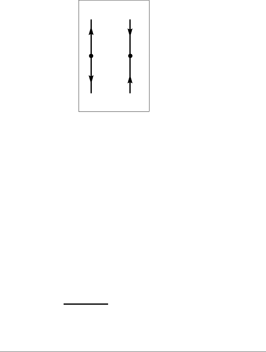
are headed. For example, Figure 7.2 (a) shows that the x-values diverge from 0

as t increases. This ﬁgure, which suppresses the t-axis, is a simple version of a

phase portrait, which we describe at length later. The idea of the phase portrait is

to compress information. The arrows indicate the direction of solutions (toward

or away from equilibria) without graphing speciﬁc values of t.Aswithmaps,we

are often primarily interested in understanding qualitative aspects of ﬁnal state

277

D IFFERENTIAL E QUATIONS

(a) (b)

Figure 7.2 Phase portraits of ˙

ⴝ

ax.

Since x is a scalar function, the phase space is the real line ⺢. (a) The direction of

solutions is away from the equilibrium for a ⬎ 0. (b) The direction of solutions is

toward the equilibrium for a ⬍ 0.

behavior. Other details, such as the rate at which orbits approach equilibria, are

lost in a phase portrait.

For a ⬍ 0, (7.6) models exponential decay, as shown in Figure 7.2(b),

and x ⬅ 0 is still an equilibrium solution. Examples include Newton’s law of

cooling, which was described above, and radioactive decay, where the mass of a

radioactive isotope decreases according to the exponential decay law. No matter

how we choose the initial condition x

, we see that x(t) tends toward 0 as time

progresses; that is, lim

t→

⬁

x(t) ⫽ lim

t→

⬁

⫽ 0. The ﬂow F(t, x

) of solutions

is shown in Figure 7.1 (b). In the phase portrait of Figure 7.2(b) we suppress t and

depict the motion of the solutions toward 0.

7.2 ONE-DIMENSIONAL NONLINEAR

DIFFERENTIAL EQUATIONS

E XAMPLE 7.3

Equation (7.6) ceases to be an appropriate model for large populations x

because it ignores the effects of overcrowding, which are modeled by non-linear

terms. It is perhaps more accurate for the rate of change of population to be a

278

7.2 ONE-DIMENSIONAL N ONLINEAR D IFFERENTIAL E QUATIONS

logistic function of the population. The differential equation

x ⫽ ax(1 ⫺ x), (7.9)

where a is a positive constant, is called the logistic differential equation.Asx gets

close to 1, the limiting population, the rate of increase of population decreases to

zero.

This equation is nonlinear because of the term ⫺ax

on the right side. Although

the equation can be solved analytically by separating variables (see Exercise 7.4),

in this section we will describe alternative methods that are geometric in nature

and that can quickly reveal some important qualitative properties of solutions.

We might ask, for example, which initial conditions yield increasing solutions?

Which yield decreasing solutions? Given an initial population, to what ﬁnal state

will the population evolve? The qualitative methods developed here are of critical

importance because most nonlinear equations are impossible to solve analytically

in closed form.

We begin by ﬁnding constant solutions of (7.9). Setting

x equal to 0 and

solving for x yields two equilibrium solutions: namely x ⬅ 0andx ⬅ 1. Figure

7.3 shows the family of solutions, or ﬂow, of (7.9). For each initial condition x

there is a single solution curve that we denote by F(t, x

) which satisﬁes (1) the

x = 0

x = 1

(a) (b)

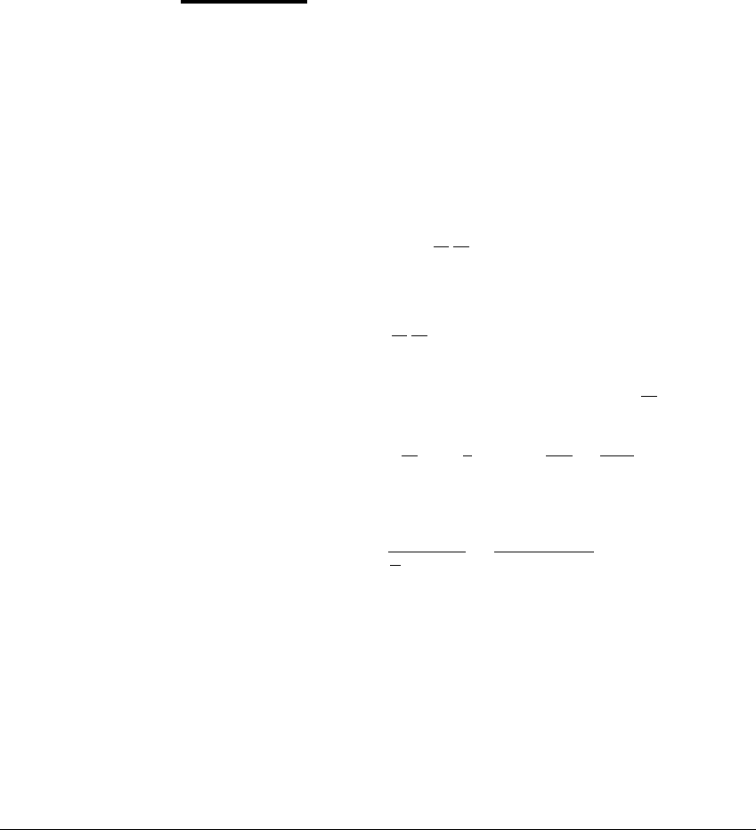
Figure 7.3 Solutions of the logistic differential equation.

(a) Solutions of the equation

x ⫽ x(1 ⫺ x). Solution curves with positive initial

conditions tend toward x ⫽ 1ast increases. Curves with negative initial condi-

tions diverge to ⫺

⬁

. (b) The phase portrait provides a qualitative summary of the

information contained in (a).

279

D IFFERENTIAL E QUATIONS

differential equation, and (2) the initial condition x

. The solution curve F(t, x

)

may or may not be deﬁned for all future t. The curve F(t, 1 2), shown in Figure

7.3, is asymptotic to the equilibrium solution x ⬅ 1, and is deﬁned for all t.On

the other hand, the curves F(t, x

) shown in the ﬁgure with x

⬍ 0 “blow up

in ﬁnite time”; that is, they have a vertical asymptote for some ﬁnite t. (Since

negative populations have no meaning, this is no great worry for the use of the

logistic equation as a population model.) See Exercise 7.4 to work out the details.

Another example of this blow-up phenomenon is given in Example 7.4.

Since we have not explicitly solved (7.9), how were we able to graph its

solutions? We rely on three concepts:

1. Existence: Each point in the (t, x)-plane has a solution passing through

it. The solution has slope given by the differential equation at that point.

2. Uniqueness: Only one solution passes through any particular (t, x).

3. Continuous dependence: Solutions through nearby initial conditions

remain close over short time intervals. In other words, the ﬂow F (t, x

)

is a continuous function of x

as well as t.

Using the ﬁrst concept, we can draw a slope ﬁeld in the (t, x)-plane by

evaluating

x ⫽ ax(1 ⫺ x) at several points and putting a short line segment with

the evaluated slope at each point, as in Figure 7.4. Recall that for an autonomous

x = 1

x = 0

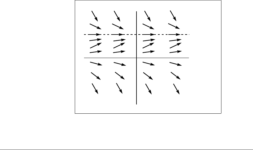
Figure 7.4 Slope ﬁeld of the logistic differential equation.

At each point (t, x), a small arrow with slope ax(1 ⫺ x) is plotted. Any solution

must follow the arrows at all times. Compare the solutions in Figure 7.3.

280

7.2 ONE-DIMENSIONAL N ONLINEAR D IFFERENTIAL E QUATIONS

equation such as this, the slope for a given x-value is independent of the t-value,

since t does not appear in the right-hand side of (7.9).

Curves can now be constructed that follow the slope ﬁeld and which, by

the second concept, do not cross. The third concept is referred to as “continuous

dependence of solutions on initial conditions”. All solutions of sufﬁciently smooth

differential equations exhibit the property of continuous dependence, which is a

consequence of continuity of the slope ﬁeld. Theorems pertaining to existence,

uniqueness, and continuous dependence are discussed in Section 7.4.

The concept of continuous dependence should not be confused with “sensi-

tive dependence” on initial conditions. This latter property describes the behavior

of unstable orbits over longer time intervals. Solutions may obey continuous de-

pendence on short time intervals and also exhibit sensitive dependence, and

diverge from one another on longer time intervals. This is the characteristic of a

chaotic differential equation.

The phase portrait of the logistic differential equation (7.9) is shown in

Figure 7.3(b). Note how the phase portrait summarizes the information about the

asymptotic behavior of all solutions. It does this by suppressing the t-coordinate.

The arrows on the phase portrait show the sign of the derivative (positive or

negative) for points between, greater than, or less than the equilibrium values.

For one-dimensional autonomous differential equations, the phase portrait gives

almost all the important information about solutions.

When an interval of nonequilibrium points in the phase portrait is bounded

by (ﬁnite) equilibria, then solutions for initial conditions in the interval converge

to one equilibrium for positive time (as t →

⬁

) and to the other for negative time

(as t → ⫺

⬁

). The latter corresponds to following all arrows in the slope ﬁeld

backwards. This fact is illustrated in Figure 7.3, and is the subject of Theorem 8.3

of Chapter 8.

As in the case of iterated maps, an equilibrium solution is called attracting

or a sink if the trajectories of nearby initial conditions converge to it. It is called

repelling or a source if the solutions through nearby initial conditions diverge

from it. Thus in (7.6), x ⬅ 0 is attracting in the case a ⬍ 0 and repelling in the

case a ⬎ 0. In (7.9), x ⬅ 0 is repelling and x ⬅ 1 is attracting.

✎ E XERCISE T7.1

Draw the slope ﬁeld and phase portrait for

x ⫽ x

⫺ x. Sketch the resulting

family of solutions. Which initial conditions lead to bounded solutions?

281

D IFFERENTIAL E QUATIONS

Next we explore the phenomenon of “blow up in ﬁnite time”. As men-

tioned above, all initial conditions that lie between two equilibria on the one-

dimensional phase portrait will move toward one of the equilibria, unless it is an

equilibrium itself. In particular, the trajectory of the initial condition will exist

for all time. The following example shows that for initial conditions that are not

bounded by equilibria, solutions do not necessarily exist for all time.

E XAMPLE 7.4

Consider the initial value problem

x ⫽ x

x(t

) ⫽ x

. (7.10)

We solve this problem by a method called separation of variables. First, divide

by x

, then integrate both sides of the equation

⫽ 1

with respect to time from t

to t:



dt ⫽



dt ⫽ t ⫺ t

. (7.11)

Making the change of variables x ⫽ x(t) means that dx replaces

dt, yielding

t ⫺ t

⫽



x(t)

x(t

)

⫽⫺



x(t)

x(t

)

⫽⫺

x(t)

⫹

x(t

)

. (7.12)

Solving for x(t), we obtain

x(t) ⫽

⫹ t

⫺ t

⫽

1 ⫹ x

⫺ t)

. (7.13)

The result is valid if x is nonzero between time t

and t.Thusx(t)musthavethe

same sign (positive or negative) as x(t

When x

⫽ 0(orwhenx ⫽ 0 at any time), the unique solution is the

equilibrium x ⬅ 0, which is deﬁned for all t. When x

⫽ 0, the solution is not

deﬁned if the denominator 1 ⫹ x

⫺ t) is 0. In this case, let t

⬁

⫽ t

⫹ 1 x

; t

⬁

the solution of 1 ⫹ x

⫺ t) ⫽ 0. Then lim

t→t

⬁

x(t) ⫽

⬁

. For x

⫽ 0, therefore,

the solution x(t) exists only for t in the interval (⫺

⬁

)or(t

⬁

), whichever

contains t

282

7.2 ONE-DIMENSIONAL N ONLINEAR D IFFERENTIAL E QUATIONS

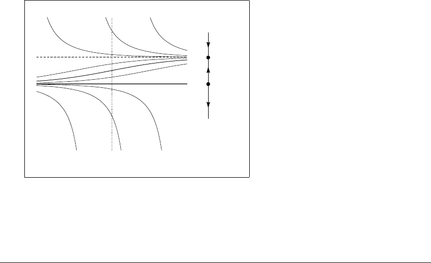
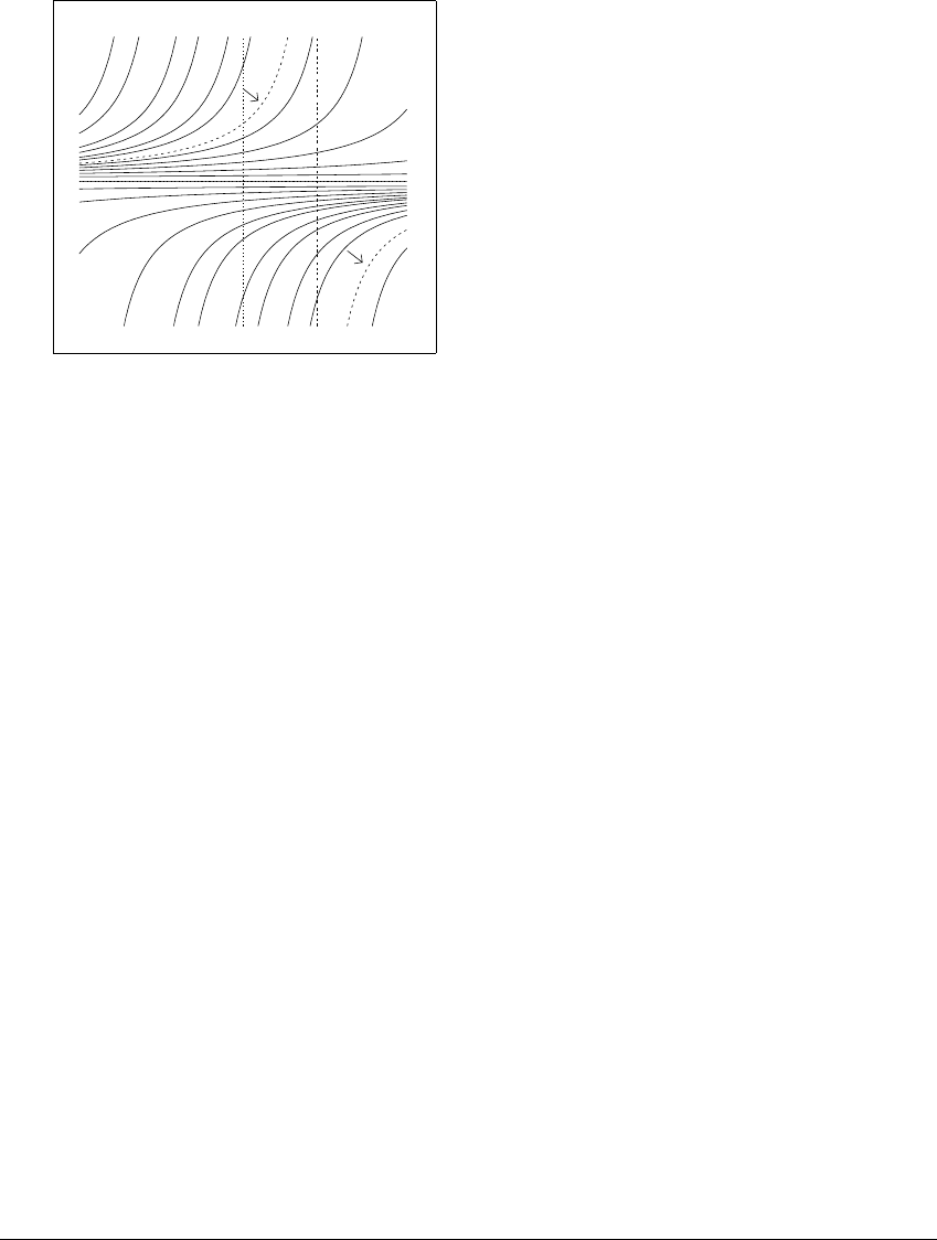
Figure 7.5 Solutions that blow up in ﬁnite time.

Curves shown are solutions of the equation

x ⫽ x

. The dashed curve in the upper

left is the solution with initial value x(0) ⫽ 1. This solution is x(t) ⫽ 1 (1 ⫺ t),

which has a vertical asymptote at x ⫽ 1, shown as a dashed vertical line on the

right. The dashed curve at lower right is also a branch of x(t) ⫽ 1 (1 ⫺ t), one that

cannot be reached from initial condition x(0) ⫽ 1.

The solution curves of (7.10) are shown in Figure 7.5. The constant x ⬅ 0is

an equilibrium. All curves above the horizontal t-axis blow up at a ﬁnite value of

t; all curves below the axis approach the equilibrium solution x ⬅ 0. For example,

if t

⫽ 0andx

⫽ 1, then t

⬁

⫽ 1, and the solution x(t) ⫽ 1 (1 ⫺ t) exists on

(⫺

⬁

, 1). This solution is the dashed curve in the upper left of Figure 7.5. Equation

(7.13) seems to suggest that the solution continues to be deﬁned on (1,

⬁

), but

as a practical matter, the solution of the initial value problem with x(0) ⫽ x

longer exists for t beyond the point where x(t)goesto

⬁

In general, notice that the solution (7.13) has 2 branches. In Figure 7.5,

arrows point to the 2 dashed branches of x(t) ⫽ 1 (1 ⫺ t). Only the branch with

x(t)andx

having the same sign is valid for the initial value problem with x

⫽ 1.

The other branch is spurious as far as the initial value problem is concerned, since

(7.12) fails to make sense when x(t

)andx(t) have opposite signs.

Solutions that blow up in ﬁnite time are of considerable interest in mathe-

matical modeling. When a solution reaches a vertical asymptote, the time interval

over which the differential equation is valid has reached an end. Either the model

needs to be reﬁned to better reﬂect the properties of the system being modeled,

or the system itself has a serious problem!

283

D IFFERENTIAL E QUATIONS

➮ COMPUTER EXPERIMENT 7.1

To do the Computer Experiments in the next few chapters, you may need to

read Appendix B, an introduction to numerical solution methods for differential

equations. A good practice problem is to choose some version of the Runge-

Kutta algorithm described there and plot solutions of the differential equations

of Figures 7.1, 7.3 and 7.5.

7.3 LINEAR DIFFERENTIAL EQUATIONS IN

MORE THAN ONE DIMENSION

So far we have discussed ﬁrst-order equations with one dependent variable. Now

we move on to more dependent variables, beginning with a system of two linear

equations. The solution of the system

x ⫽ 2x

y ⫽⫺3y (7.14)

can be determined by solving each equation separately. For an initial point (x

)

at time t ⫽ 0, the solution at time t is the vector (x

⫺3t

Figure 7.6 shows a graphical representation of the vector ﬁeld of (7.14). A

vector ﬁeld on ⺢

is a function that assigns to each point in ⺢

an n-dimensional

vector. In the case of a differential equation, the coordinates of the vector assigned

to point (x, y) are determined by evaluating the right side of the equation at (x, y).

For (7.14), the vector (2x, ⫺3y) is placed at the point (x, y), as seen in Figure

7.6(a). As in the case of slope ﬁelds, these vectors are tangent to the solutions.

Thus the vector (2x, ⫺3y) gives the direction the solution moves when it is at

the point (x, y). The length |(2x, ⫺3y)| of the vector is the speed of the solution

as it moves through the point.

Since (7.14) is autonomous, (the variable t does not appear explicitly on

the right side of (7.14)), the vector assigned to (x, y) is independent of time.

A solution passing through (x, y)atonetimet will not go a different direction

or speed when passing through (x, y) at a different time. Autonomous equations

have a particularly useful property that enables us to draw phase portraits for these

systems: graphs of solutions (x(t),y(t)) drawn in the xy-plane, ignoring the t-axis,

do not cross. (This property holds in addition to the fact that they do not cross in

(x, y, t)–space, which is a consequence of uniqueness of solutions.) Figure 7.6(b)

284

7.3 LINEAR D IFFERENTIAL E QUATIONS IN M ORE THAN O NE D IMENSION

(a) (b)

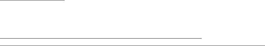
Figure 7.6 Vector ﬁeld and phase plane for a saddle equilibrium.

(a) The vector ﬁeld shows the vector (

y) at each point (x, y) for (7.14). (b) The

phase portrait, or phase plane, shows the behavior of solutions. The equilibrium

(x, y) ⬅ (0, 0) is a saddle. The time coordinate is suppressed in a phase portrait.

shows the phase portrait of solutions of (7.14). A phase portrait in two dimensions

is often called a phase plane, and in higher dimensions it is called phase space.

The dimension of the phase space is the number of dependent variables. Arrows

on the solution curves in phase space indicate the direction of increasing time.

The system (7.14) is uncoupled, meaning that neither of the dependent

variables appear in the other’s equation. More generally, the equation has the

form

˙v ⫽ Av, (7.15)

where v is a vector of variables, and A is a square matrix. Since the right-hand

side of (7.15) is the zero vector when v ⫽ 0, the origin is an equilibrium for

(7.15). The stability of the equilibrium can be determined by the eigenvalues of

the matrix of coefﬁcients.

E XAMPLE 7.5

We show how eigenvalues are used to ﬁnd the solution v ⫽ (x, y)of

x ⫽⫺4x ⫺ 3y

y ⫽ 2x ⫹ 3y (7.16)

285

D IFFERENTIAL E QUATIONS

with initial value v(0) ⫽ (1, 1). In vector form, (7.16) is given by (7.15) where

v ⫽





and A ⫽



⫺4 ⫺3



The eigenvalues of the matrix A are 2 and ⫺3. Corresponding eigenvectors

of A are (1, ⫺2) and (3, ⫺1), respectively. We refer the reader to Appendix A

for fundamentals of eigenvalues and eigenvectors.

For a real eigenvalue

␭

of A, an associated eigenvector u has the prop-

erty that Au ⫽

␭

u. Set v(t) ⫽ e

␭

u. By deﬁnition of eigenvector, Av (t) ⫽

␭

Au ⫽ e

␭

(

␭

u). Since u is a ﬁxed vector, ˙v(t) ⫽

␭

u as well. Each eigenvalue-

eigenvector pair of A leads to a solution of ˙v ⫽ Av. As the phase plane in

Figure 7.7 shows, any vector along the line determined by an eigenvector u is

stretched or contracted as t increases, depending on whether the corresponding

eigenvalue

␭

is positive or negative. The phase plane of (7.16) is similar to that

of (7.14) except that lines in the direction of the eigenvectors u

⫽ (1, ⫺2) and

⫽ (3, ⫺1) take the place of the x and y axes, respectively. Both v(t) ⫽ e

␭

and v(t) ⫽ e

␭

are solutions.

If this vector argument is not clear, write the vectors in coordinates. Since

⫽ (1, ⫺2), the corresponding solution v(t) ⫽ (x(t),y(t)) is (1e

␭

, ⫺2e

␭

Differentiating each coordinate separately gives (1

␭

, ⫺2

␭

), which is

␭

v(t), as needed. The same argument works for u

.When

␭

⫽

␭

, then u

and u

are linearly independent, and the general solution of ˙v ⫽ Av is given by

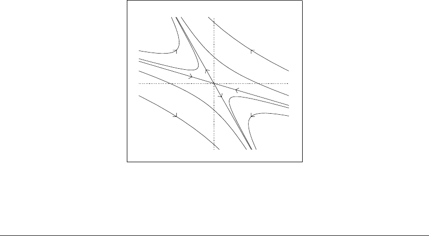
Figure 7.7 Phase plane for a saddle equilibrium.

For (7.16), the origin is an equilibrium. Except for two solutions that approach the

origin along the direction of the vector (3, ⫺1), solutions diverge toward inﬁnity,

although not in ﬁnite time.

286