Baker K.R. Optimization Modeling with Spreadsheets

Подождите немного. Документ загружается.

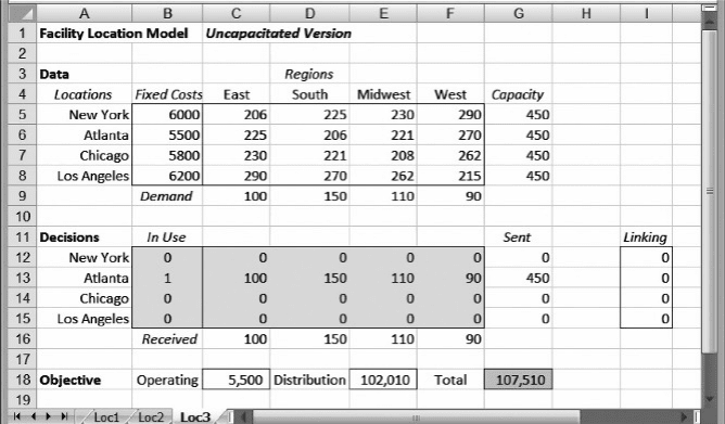
The streamlined version, shown in Figure 7.11, ﬁnds the same optimal solution

with a model formulation that contains half as many constraints. The speciﬁcation

of the problem is as follows.

Objective: G18 (minimize)

Variables: B12:F15

Constraints: C16:F16 ≥ C9:F9

I12:I15 ≤ 0

B12:B15 = binary

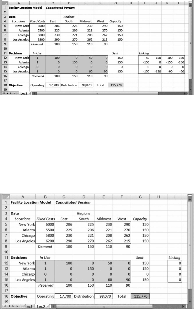
Figure 7.10. Optimal solution for Example 7.3.

Figure 7.11. Alternative model for Example 7.3.

266 Chapter 7 Integer Programming: Logical Constraints

Two changes from the previous model are present. First, no explicit capacity con-

straints appear because these are combined with the linking constraints. Second,

one linking constraint appears (cells I12:I15) for each potential DC location, rather

than one for each combination of DC location and sales region. Its left-hand side is

expressed in the form



– C

The facility location model can be thought of as the strategic version of the trans-

portation problem, in the sense that the warehouse or DC locations are treated as given

in the transportation problem but as choices in the facility location problem.

Associated with these choices are the ﬁxed costs of operating a facility, and these

costs are incorporated into the model with the help of linking constraints.

7.4.2. Uncapacitated Version

In the classical uncapacitated facility location problem, no capacity constraints are

associated with the potential facility locations. In a supply-chain design setting, this

might be the case if capacities are completely ﬂexible and can be determined after

the facility locations are selected. The model of the capacitated case can be adapted

to the uncapacitated case in different ways.

Perhaps the simplest way to represent the uncapacitated version of the model is to

use the capacitated version with very large capacities. For example, the capacity at

each facility location could be set equal to the sum of all demands. In symbols, this

means setting



In this formulation, capacity constraints do not inhibit the selection of facility locations

based on cost, and the linking constraints ensure correct accounting for the ﬁxed oper-

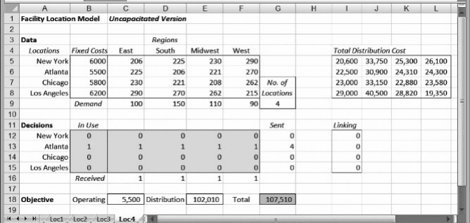
ating costs. Figure 7.12 shows the corresponding spreadsheet layout. The only change

(in the streamlined version) from the formulation of the capacitated model is the value

of 450, which appears in the role of capacity, in the range G5:G8. When we optimize

this model, we ﬁnd that the minimum cost drops to $107,510, as shown in Figure 7.12,

and that the optimal conﬁguration is to use only the Atlanta location. Without capacity

constraints, we anticipate that the optimal cost should be lower than the optimal cost

for the capacitated model. However, it may be surprising to ﬁnd that the complete

relaxation of the capacity constraints leads to modest savings. Compared to the capaci-

tated version, the uncapacitated conﬁguration saves $8260 (¼ 115,770 2 107,510) or

about 7 percent.

An alternative modeling approach is based on an insight about the nature of opti-

mal transportation patterns in the uncapacitated case. In the capacitated model of

Figure 7.11, for example, Midwest demand is met from two sources—New York

and Los Angeles. This kind of split would not occur in an optimal solution to the unca-

pacitated version of the problem because there is never an incentive to meet demand

from two sources. In the example, it is cheaper to supply Midwest sales from

New York than from Los Angeles, so there would be no reason to ship from Los

Angeles to the Midwest. (In fact, if the Atlanta location is in use, there is no reason

7.4. Linking Constraints: The Facility Location Model 267

to ship from New York, either.) A general property of the uncapacitated model is that

an optimum exists in which each demand is met from just one source. In particular,

demand should be met from the least expensive source among the facility locations

in the solution. Therefore, we don’t really need the x

variables. Instead, we can deﬁne

= 1 if facility i serves demand j

= 0 otherwise

In words, u

indicates whether demand in region j is met from facility i. When u

¼ 1,

we know that the corresponding distribution cost must be equal to (c

, since the

entire demand quantity d

will be met from the one source. Accordingly, the (stream-

lined) formulation takes the following form.

Minimize z =



subject to



≥ 1(7.6)



≤ ny

(7.7)

The number (n) of demand regions appears in (7.7) because it is the largest possible

value for the sum on the left-hand side. Finally, although the variables u

take on

values of zero or one, we do not have to declare them as binary because the

Figure 7.12. Optimal solution for the unconstrained model.

268 Chapter 7 Integer Programming: Logical Constraints

optimization will always lead to a 0-1 solution when the u

are treated as continuous

variables. Thus, we specify the model in Figure 7.13 as follows.

Objective: G18 (minimize)

Variables: B12:F15

Constraints: C16:F16 ≥ 1

I12:I15 ≤ 0

B12:B15 = binary

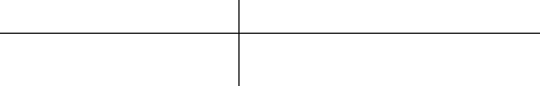
Figure 7.13 displays an optimal solution for the spreadsheet containing

the alternative unconstrained model. We can conﬁrm the optimal total cost of

$107,510, and an opti mal design calling for a facility in Atlanta to supply the entire

set of demands. In the spreadsheet, the following changes have been made from the

model in Figure 7.12.

†

The “very large” capacities formerly in cells G5:G8 are no longer needed.

†

The Sent totals now show the number of regions served from a warehouse rather

than the quantity shipped.

†

A typical linking constraint follows the form of (7.7). For example, the formula

in cell I12 is now

=G12–$G$9

∗

$B12.

†

The Total Distribution Cost array in I5:L8 holds the terms (c

) from the

objective function. These are calculated from the original array of unit

costs and demands in each region. Then, the Distribution component of

total cost in cell E18 is calculated with the Excel formula

=SUMPRODUCT(I5:L8,C12:F15).

The uncapacitated facility location problem is sometimes just the central portion

of a larger and more complicated design problem. One reason why it is desirable to use

Figure 7.13. Optimal solution for the alternative unconstrained model.

7.4. Linking Constraints: The Facility Location Model 269

variables in the formulation is that other kinds of constraints, particularly logical

conditions, may apply to the potential facility locations. For example, suppose we

want to distribute to at most one customer location from New York. To achieve this

requirement, add the constraint u

+ u

≤ 1. As discussed earlier in

the chapter, logical constraints can often be developed in linear form with the help

of binary variables, or at least variables that behave as if they were binary.

We have examined two alternative modeling approaches to both the capacitated

and uncapacitated problems. These alternatives are based on the streamlined linking

constraint, using (7.5) in place of (7.3). One advantage of the streamlining is that

there are fewer elements on the spreadsheet, so the model is easier to build and

debug. However, there is a potential downside. The streamlined version may require

more computational effort than the original version to locate an optimum. This differ-

ence could be important in larger models, with perhaps dozens of facility locations and

hundreds of customer demands.

7.5. DISJUNCTIVE CONSTRAINTS: THE MACHINE

SEQUENCING PROBLEM

Scheduling and sequencing problems are notoriously difﬁcult to solve, but some

progress is possible with the use of integer programming. In the basic machine-

sequencing problem, one processor (or machine) is available to process several

jobs. The jobs are all ready for processing at the outset (time zero), but the machine

can accommodate only one job at a time. The jobs are described by a processing

time ( p

for job j) and a due date (d

Depending on the sequence chosen, job j will start processing at time s

and com-

plete its processing at time s

+ p

. If a job completes after its due date, then the job is

said to be tardy, and its tardiness is measured by (s

+ p

)–d

. On the other hand, if a

job completes on or before its due date, then the job is on time, and its tardiness is zero.

In other words, a job’s tardiness may be zero, but it can never be negative. One way

of measuring schedule performance is to sum the tardiness of all jobs, thus computing

the total tardiness in the schedule. A common objective in scheduling is to minimize

total tardiness, as a means of quantifying the effectiveness of a schedule at meeting

due dates. The use of total tardiness as a performance measure prevents one job’s

earliness from offsetting another’s lateness, thereby focusing attention on jobs that

miss their due dates. Obviously, when total tardiness is zero, this means that all due

dates have been met.

As an example, Miles Manufacturing faces a version of the machine sequencing

problem.

EXAMPLE 7.4

Miles Manufacturing Company

Miles Manufacturing Company is a regionally focused production shop that fabricates metal

components for auto companies. Its scheduling efforts center around a large piece of equipment

that handles a variety of operations, such as drilling, shaping, polishing, and mechanical testing.

270 Chapter 7 Integer Programming: Logical Constraints

Work arrives at the machine in batches—each batch corresponding to a customer order—and the

information system provides data on the size of the order, how long it will take to process, and

when it is due (the due dates having been previously negotiated with customers). These due

dates, which apply to completion in the shop, are adjusted for the delivery time needed to put

the completed order in the customer’s hands. When several orders are waiting to be processed,

the supervisor looks for guidance on how the orders should be sequenced. The minimization of

total tardiness is an accepted criterion for a schedule.

This morning’s workload consists of six jobs, as described in the following table.

Job number 1 2 3 4 5 6

Processing time (hours) 5 7 9 11 13 15

Due date (hours from now) 28 35 24 32 30 40

The problem is to sequence the six jobs so that work can begin. With 60 total hours of work to

schedule, and a latest due date of 40, it is obvious that the jobs cannot all be ﬁnished on time, and

some tardiness will occur even in the best schedule. B

The optimization problem is to select a sequence for the jobs that minimizes total

tardiness. For decision variables we can use the job start times, s

. The key feasibility

constraints reﬂect the fact that, for any pair of jobs j and k, either k follows j or else

j follows k. In other words, either job j completes before k starts, or else job k com-

pletes before j starts. In symbols, either

+ p

≤ s

or s

+ p

≤ s

These are called disjunctive constraints, meaning that one or the other—but not

both—must hold for a solution to be feasible. To represent this requirement in an

integer program, we use the following pair of constraints

+ p

≤ s

+ M(1 − y

)

+ p

≤ s

+ My

where y

is a binary variable and M represents a nonrestrictive large value, such as the

sum of all the processing times. When y

¼ 1, the ﬁrst constraint forces the start of job

k to be at least as late as the completion of job j, and the second constraint does not

restrict the choice of variables. On the other hand, when y

¼ 0, the ﬁrst constraint

does not restrict the choice of variables, and the second constraint forces the start of

job j to be at least as late as the completion of job k. In other words

= 1 if job k follows job j, and zero otherwise.

= 1 if job j follows job k, and zero otherwise.

We can also rewrite the constraint pair with all variables moved to the left-hand

side and parameters on the right-hand side, thus obtaining the following pair of con-

straints

− s

+ My

≤ M − p

− s

+ My

≥ p

7.5. Disjunctive Constraints: The Machine Sequencing Problem 271

Expressed this way, the left-hand sides of these conditions are identical, which allows

for some efﬁciency in building the spreadsheet model. In addition to the disjunctive

constraints, we need constraints that track the tardiness of job j, which is denoted

by t

. This can be accomplished by treating t

as a nonnegative decision variable

and imposing the following constraint

≥ s

+ p

− d

When job j is on time, the right-hand side of this constraint will be negative or zero, so

the tardiness variable t

will become zero because all variables are nonnegative by

assumption. Otherwise, the constraint will be tight (because the objective is to

make total tardiness as small as possible), and the tardiness variable t

will be equal

to the right-hand side. We can also write th is constrai nt with decision variables on

the left and parameters on the rig ht, as follows

− t

≤ d

− p

An algebraic statement of the entire model follows.

Minimize z =



subject to:

− s

+ My

≤ M − p

, for all job pairs j , k

− s

+ My

≥ p

, for all job pairs j , k

− t

≤ d

− p

, for all jobs j

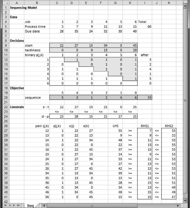
A spreadsheet model for Miles Manufacturing is shown in Figure 7.14. The ﬁrst

module of the spreadsheet contains the data for the problem. The next module contains

the three types of decision variables: start times (s

), tardiness values (t

), and binary

variables ( y

, needed only for j , k). As usual, the decision variables are highlighted.

The third module is a one-cell module containing the objective function, which is just

the sum of the job tardiness values.

Although we need the variables y

only for j , k, the worksheet also shows y

for

j . k. In the worksheet, these values are not highlighted, signifying that they are not

decision variables. Instead, their values are calculated directly from the decision vari-

ables. For example, once we know the value of y

, then it follows that y

is its binary

complement.

The last module contains the constraints of th e problem. First, we see the LT

inequalities s

– t

≤ d

– p

. These are expressed in rows 22– 24, in the columns cor-

responding to the respective jobs. Next, we see the disjunctive constraints in rows

27–41. Each row contains a disjunctive pair, one expressed as an LT constraint and

the other expressed as a GT constraint, each with the same left-hand side. The left-

hand side appears in column G, while the right-hand sides appear in columns I and K.

272

Chapter 7 Integer Programming: Logical Constraints

We specify the problem as follows.

Objective: I18 (minimize)

Variables: C9:H10,D12:H12,E13:H13,F14:H14,G15:H15,H16

Constraints: C22:H22 ≤ C24:H24

G27:G41 ≥ I27:I41

G27:G41 ≤ K27:K41

D12:H12 = binary

E13:H13 = binary

F14:H14 = binary

G15:H15 = binary

H16 = binary

Figure 7.14. Spreadsheet model for Example 7.4.

7.5. Disjunctive Constraints: The Machine Sequencing Problem 273

The worksheet in Figure 7.14 contains an optimal sequence. Although the order

of the start times tells us that an optimal sequence is given by 5-3-1-2-4-6, we can also

determine the sequence from the full array of y

values. In cells I12– I17, we sum the

entries in the corresponding row of the array. This value tracks the number of jobs

following the job in that row. For example, three jobs come after job 1, indicating

that job 1 is third in sequence. We can then construct the optimal sequence in row

20 by using these numbers and the MATCH function. Thus, after downloading

processing times and due dates from the central information system and then using

an integer programming model, Miles Manufacturing can construct optimal sequences

on the supervisor’s spreadsheet.

The sequencing model is more general than Example 7.4 might suggest

because it can accommodate other objective functions as well. For example, instead

of minimizing the total tardiness in the schedule, we might instead want to minimize

the number of tardy jobs. In other situations, there could be a contractual penalty deter-

mined by a job’s delay, and the criterion could be minimization of delay penalties.

Sequencing problems with a variety of criteria can ﬁt into this framework, where dis-

junctive constraints enable the problem to be solved as an integer linear program.

More generally, disjunctive constraints are appropriate whenever we encounter

situations in which we want at least one constraint out of a pair to apply. Suppose

we have a pair of LT constraints in our model

LHS

≤ RHS

LHS

≤ RHS

Suppose also that we wish to have at least one of these two constraints satisﬁed. We

can then represent the two constraints in our model as follows.

LHS

≤ RHS

+ My

LHS

≤ RHS

+ M(1 − y)

With the additional terms, the binary variable y determines which constraint will be

met automatically. When y ¼ 1, the right-hand side of the ﬁrst constraint becomes

quite large, and the constraint is satisﬁed for any choice of the other variables in the

model. The right-hand side of the second constraint is unaffected, so the other vari-

ables must be chosen to be feasible in that constraint. When y ¼ 0, the right-hand

side of the second constraint becomes quite large, and the other variables must be

chosen to be feasible in the ﬁrst constraint.

7.6. TOUR AND SUBSET CONSTRAINTS: THE

TRAVELING SALESPERSON PROBLEM

In the traveling salesperson problem (TSP), a sales rep has several customers to visit,

each in a separate city. The sales rep knows the distances between pairs of cities and

must plan a trip that visits each of the cities once and returns home. This type of trip is

called a tour. Speciﬁcally, the sales rep would like to plan a tour that has the minimum

total distance.

274

Chapter 7 Integer Programming: Logical Constraints

The given information in the TSP is an array of distances. In the literal version of

the problem, we might expect the distances to be symmetric—that is, the distance from

A to B should be the same as the distance from B to A. However, there are applications

where the distances need not be symmetric. For example, a paint booth may or may not

need cleaning between two successive products on the production line. If two succes-

sive items use the same color of paint, then there is no cleaning required. But if the

items require different colors, then there is a need to clean out the painting equipment.

The time required depends on the paint color just ﬁnishing and on the paint color about

to begin. The ( i, j)th entry in the data array represents the time required to clean the

equipment between color i and color j, and it need not be the same as the cleaning

time between j and i. In a complete cycle through the products, with one batch for

each color, the painting time is ﬁxed, but the length of the schedule is minimized

when the total cleaning time is minimized. Total cleaning time is in turn the total

length of a tour in the array of cleaning times. As an example, consider the Douglas

Electric Cart Company.

EXAMPLE 7.5

Douglas Electric Cart Company

The Douglas Company assembles small electric vehicles which are sold for use on golf courses,

at university campuses, and in sports stadiums. In these markets, customers like to buy in a var-

iety of colors, so Douglas offers several choices. As a result, its manufacturing operations

include a sophisticated painting operation, which is separately scheduled.

Today’s schedule contains six colors (C1–C6) with cleaning times as shown in the table

below.

C1 C2 C3 C4 C5 C6

C1 –16632120 6

C2 57 – 40 46 69 42

C3 23 11 – 55 53 47

C4 71 53 58 – 47 5

C5 27 79 53 35 – 30

C6 57 47 51 17 24 –

The entry in row i and column j of the table gives the cleaning time required between product

lots of color Ci and color Cj. Each production run consists of a cycle through the full set of

colors, and the operations manager wishes to sequence the colors so that the total cleaning

time in a cycle is minimized. B

Returning to the traveling salesperson terminology, we refer to the colors in a pro-

duction cycle as cities, and we refer to the cleaning time objective as the total distance.

For example, if the painting schedule calls for the color sequence given by the cycle

1-2-3-4-5-6-1

then the total distance (cleaning time in the cycle) is 16 + 40 + 55 + 47 + 30 +

57 ¼ 245. We would like to know whether this is the minimum.

7.6. Tour and Subset Constraints: The Traveling Salesperson Problem 275