Baker K.R. Optimization Modeling with Spreadsheets

Подождите немного. Документ загружается.

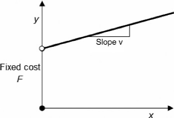
Alternativel y, using symbols, we write

TC = Fy + vx

where F represents the ﬁxed cost and v represents the unit (variable) cost. A sketch of

the total cost function is shown in Figure 7.4. The variables x and y are decision vari-

ables, wh ere x is a normal (continuous) variable and y is a binary variable. Constraints

in the linear program involve only the variable portion—that is, they involve only the

variable x, not the variable y. We also want the variables x and y to work consistently.

Speciﬁcally, we want to ensure that y ¼ 1 (so that we incur the ﬁxed cost) whenever

x . 0, and we want to have y ¼ 0 (so that we avoid ﬁxed cost) when x ¼ 0. To achieve

consistency in the two variables, we add the following linking constraint.

x ≤ My

where M represents some upper bound on the variable x.

To appreciate the linking constrai nt, imagine that Solver approaches the selection

of variables in two stages. In the ﬁrst stage, bi nary variables (such as y) are set to either

0 or 1; then, in the second stage, continuous variables (such as x) are determined. The

two ﬁrst-stage choices for the variable y provide us with the following possibilities in

the linking constraint

y = 1 so that x ≤ My becomes x ≤ M (meaning: x can be anything)

y = 0 so that x ≤ My becomes x ≤ 0 (meaning: x must be zero)

Thus, the variable x will be treated in a consistent way with the choice of y.In

particular, it is not possible to have y ¼

0 and x . 0. In words, we cannot avoid the

ﬁxed cost if we wish to use x at a nonzero level.

In principle, the linking constraint does allow us to set y ¼ 1 and x ¼ 0. That is,

the model permits us to incur the ﬁxed cost even without using the variable x.

However, Solver will not produce such a solution because it would always be less

costly to set y ¼ 0 and avoid the ﬁxed cost completely.

As an example of the ﬁxed cost structure, consider the product planning decision

at the Moore Ofﬁce Products Company.

Figure 7.4. Total cost with ﬁxed and variable components.

256 Chapter 7 Integer Programming: Logical Constraints

EXAMPLE 7.2

Moore Ofﬁce Products Company

Moore Ofﬁce Products has been producing and selling its goods in three product families (F1,

F2, and F3) and planning for those products using a product-mix type of linear programming

model. Each product family requires production hours in each of three departments. In addition,

each family requires its own sales force, which must be supported no matter how large or small

the sales volume happens to be. The parameters describing the situation are summarized in the

following table. Moore’s management is wondering whether it should continue to market all

three product families.

Hours required/1000 units family

Hours

F1 F2 F3 available

Department A 3 4 8 2000

Department B 3 5 6 2000

Department C 2 3 9 2000

Proﬁt per unit ($) 1.20 1.80 2.20

Sales cost ($000) 60 200 100

Demand (000s) 300 200 50

At the heart of this situation lies a decision problem analogous to the product mix

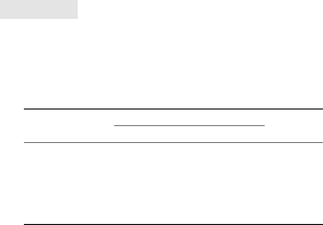
example introduced in Chapter 2. The linear programming representation of the pro-

duct mix problem, without the ﬁxed costs, is shown in Figure 7.5. By deﬁning the x-

values in thousands, we have scaled the model so that the objective function is in thou-

sands of dollars. The optimal product mix calls for producing all three families, with

F1 and F2 at their demand ceilings, and F3 at a volume of 50,000. This product mix

creates $758,000 in variable proﬁts, as computed in cell F8. If we subtract the total

ﬁxed costs of $360,000, as computed in cell F17, we are left with a net proﬁt of

$398,000, as computed in cell F19.

The linear programming solution might represent the situation in a ﬁrm that has

introduced and supported various new products over the years and now ﬁnds itself car-

rying out activities in three existing markets. The linear programming framework

suggests how to allocate capacity, provided that all three of the product families are

active. However, because ﬁxed-cost considerations are not part of the linear program-

ming analysis, we have no basis for determining whether any one of the families

should be dropped. To make the model suitable for decisions of this kind, we must

integrate the implications for ﬁxed costs.

To formulate the full problem at Moore Ofﬁce Products as an integer program-

ming model, we make two changes in the product mix formulation. First, we write

the objective function with terms for both variable proﬁt and ﬁxed cost, as follows

Net profit = 1.20x

− 60y

+ 1.80x

− 200y

+ 2.20x

− 100y

where x

represents the volume for family j, in thousands, and

= 1ifx

is positive (and the fixed cost is incurred)

= 0ifx

is zero (and the fixed cost is avoided)

7.2. Linking Constraints: The Fixed Cost Problem 257

Net proﬁt is measured in thousands due to the scaling of the x-variables and the scaling

of the ﬁxed cost coefﬁcients.

Next, we add linking constraints to ensure consistency between each of the

x– y pairs.

− My

≤ 0

− My

≤ 0

− My

≤ 0

Now we need to identify a large number to play the role of M. Essentially, we need a

number large enough that it will not limit the choice of these variables in any of the

other (demand and supply) constraints. For example, a value of 300 (thousand)

would work, since that represents the largest demand ceiling, and none of the volumes

could ever be larger.

Thus, when y

¼ 1, the linking constraint for family F2 becomes x

≤ 300; and

when y

¼ 0, the constraint becomes x

≤ 0. Similar interpretations apply to families

F1 and F3. These are valid linking constraints, but we can streamline the model

slightly. Instead of retaining separate constraints to represent the demand ceilings

and the linking relationships, we can let the linking constraint do “double duty” if

we choose a different value of M for each family and set it equal to the corresponding

demand ceiling. For example, the value of M selected for the F2 constraint could be

200 instead of 300. Then, when y

¼ 1, the constraint on the production volume for

Figure 7.5. Solution to Example 7.2 without ﬁxed costs.

258 Chapter 7 Integer Programming: Logical Constraints

family F2 becomes x

≤ 200, which also serves as a demand ceiling. When y

¼ 0, the

constraint still becomes x

≤ 0, in which case the speciﬁc choice of M does not matter.

The streamlined model, in its entirety, is the following

Maximize z = 1.20x

− 60y

+ 1.80x

− 200y

+ 2.20x

− 100y

subject to:

+ 4x

+ 8x

≤ 2000

+ 5x

+ 6x

≤ 2000

+ 3x

+ 9x

≤ 2000

− 300y

≤ 0

− 200y

≤ 0

− 50y

≤ 0

There are different ways to lay this model out in a spreadsheet. We could, for

instance, treat the xs and ys as six distinct variables and, in the traditional format,

build the spreadsheet with six columns on the left-hand side of the constraints.

Then, we could represent the constraints in the traditional format, as six rows, with

the usual SUMPRODUCT functions. An alternative is to pair the xs and ys that are

linked in successive rows, using just three columns (one for each product family).

Then we could associate the linking constraints with variable pairs and display

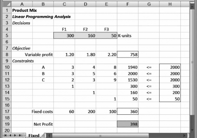
them in columns (one for each product family). Figure 7.6 shows the traditional

layout, and Figure 7.7 shows the alternative. In the latter, formulas in cells C16:E16

compute the left-hand side of the linking constraints. For example, the formula in

cell C16 reads:

¼ C5–C15

∗

C6.

Figure 7.6. Spreadsheet layout for Example 7.2.

7.2. Linking Constraints: The Fixed Cost Problem 259

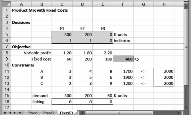
For the layout in Figure 7.7, we specify the model as follows.

Objective: F9 (maximize)

Variables: C5:E6

Constraints: F11:F13 ≤ H11:H13

C16:E16 ≤ 0

C6:E6 = binary

The optimal solution achieves a net proﬁt of $460,000, which we can obtain by

setting the Integer Tolerance to zero. In order to attain this level of proﬁts, Moore

Ofﬁce Products must forego production of product family F3 and produce families

F1 and F2 up to their respective ceilings. In other words, the model detects that

family F3 does not pay its own way and that proﬁts would be increased by not produ-

cing or selling that family at all. By using an integer programming model that incor-

porates ﬁxed costs, Moore Ofﬁce Products can conside r the implications of dropping a

product family. Such a possibility may be inﬂuenced by factors beyond proﬁts in the

coming year, but the model helps to shape and quantify the economic considerations.

7.3. LINKING CONSTRAINTS: THE THRESHOLD

LEVEL PROBLEM

Sometimes we encounter situations where, in order to do business, we are required to

participate at a speciﬁed minimum level. In purchasing, for example, we might be able

to qualify for a discounted price if we buy in quantity. Thus, a condition in the problem

Figure 7.7. Alternative layout for Example 7.2.

260 Chapter 7 Integer Programming: Logical Constraints

dictates that a decision variable must be either zero or at least as large as a speciﬁed

threshold.

The existence of a threshold level does not require an alteration in the objective

function of a model, and it can be represented in the constraints with the help of

binary variables. Suppose we have a variable x that is subject to a speciﬁed minimum

requirement. Let m denote the threshold value of x if it is nonzero. Then we can capture

this structure in an integer programming model by including the following pair of

constraints

x ≥ my

x ≤ My

where, as before, M is a large number that is greater than or equal to any value x could

feasibly take. To see how these two requirements work, again imagine that Solver

approaches the selection of variables in two stages. In the ﬁrst stage, the binary vari-

able y is set to either 1 or to 0; then, in the second stage, Solver determines x. The two

ﬁrst-stage choices for the variable y provide us with the following possibilities in the

linking constraints.

y = 1 so that: x ≥ my becomes x ≥ m (meaning: x meets the threshold)

and: x ≤ My becomes x ≤ M (meaning: x can be anything)

y = 0 so that: x ≥ my becomes x ≥ 0 (meaning: x must be nonnegative)

and: x ≤ My becomes x ≤ 0 (meaning: x must be nonpositive)

Thus, when y ¼ 1, the constraints reduce to m ≤ x ≤ M, so that x must at least meet the

threshold level. When y ¼ 0, the constraints reduce to x ¼ 0. Thus, the pair x

and y will

behave consistently, and the threshold requirement will be respected.

As a brief illustration, suppose that in Example 7.2, materials for product family

F2 can be ordered from a major supplier only if the order supports an output level of

125 (thousand) or more. The model would need two constraints, as follows

≥ 125y

≤ 200y

This pair of linking constraints ensures that if x

. 0, then it must lie between 125

and 200.

7.4. LINKING CONSTRAINTS: THE FACILITY

LOCATION MODEL

In designing its distribution system, a ﬁrm wants to know how many distribution facili-

ties it should have and where they should be located. If we think about the “how many”

question, we can see a basic tradeoff. As the ﬁrm uses more and more facilities, it can

place the facilities close to customer locations and thus reduce its variable distribution

costs. However, larger overhead costs will occur due to operating a larger number of

7.4. Linking Constraints: The Facility Location Model 261

facilities. In the other direction, as the ﬁrm uses fewer and fewer facilities, it will

encounter larger and larger variable costs, but the costs of operating the facilities

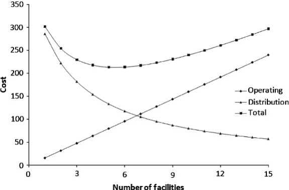
will drop. Figure 7.8 shows this tradeoff graphically. The horizontal axis represents

the number of facilities in the system. As this number increases, the total cost of dis-

tribution drops, while the cost of operating the facilities increases. (The graph shows

this latter component as a straight line, as if each facility incurs the same operating cost,

but this is only for illustration.) The total cost in the problem is the sum of distribution

cost and operating cost, shown as the U-shaped function on the graph.

The graph in Figure 7.8 is only a conce ptual device to illustrate the main tradeoff

affected by the number of locations. Important details remain. For example, once we

choose the number of facilities, we must then determine which facilities to use.

Similarly, once we choose the facilities, we must still determine how to distribute

from those facilities to the customer locations in the most desirable way. This last pro-

blem we can now recognize as a transportation problem, which we examined in

Chapter 3. Thus, the graph hides two embedded problems: (1) selecting k out of the

m possible locations for facilities in the network and, (2) solving the transportation

problem that arises once the locations are selected.

This type of tradeoff arises in several situations, but perhaps the most familiar

application relates to the location of facilities in a distribution supply chain. For this

reason, the problem is known as the facility location problem (or sometimes, the

plant location problem, or the warehouse location problem). The essential tradeoff bal-

ances the ﬁxed costs of operating discrete sources with the variable costs of providing

service from those sources. In the examples that follow, we distinguish between the

capacitated and uncapacitated version of the problem. The integer programming

model itself represents a variation on the incorporation of ﬁxed costs and the use of

linking constraints.

Figure 7.8. Cost Tradeoff in facility location.

262 Chapter 7 Integer Programming: Logical Constraints

7.4.1. Capacitated Version

In the classical capacitated facility location problem, the system contains m potential

facility locations and n existing customer demand locations. For facility location i,we

know the capacity (denoted C

) and the ﬁxed cost of operating the facility (F

). For each

customer location, we know the demand (d

) and the unit distribution cost (c

) associ-

ated with satisfying demand at location j from capacity at facility i. In this problem

statement, we typically choose a time period, such as a month or a year, as the basis

for the facility costs and the demand quantities. For decision variables, we deﬁne

= quantity sent from facility i to customer location j

= 1 if facility i is used in the design

= 0 otherwise

Then the optimization problem can be formulated algebraically as follows.

Minimize z =



subject to



≥ d

(7.1)



≤ C

(7.2)

≤ C

(7.3)

As stated, the problem contains a transportation model, represented by constraints

(7.1) and (7.2), along with the linking constraints in (7.3). The linking constraints

ensure that if we distribute from facility location i (i.e., x

. 0 for some j), then we

incur the corresponding ﬁxed cost F

in the objective function (by forcing y

to be

1). Conversely, if we want to avoid the ﬁxed cost F

, then we must have y

¼ 0,

which prevents the use of facility location i.

The model contains mn variables x

along with m variables y

, for a total of

m(n + 1) variables. There are n constraints of type (7.1), m constraints of type (7.2),

and mn constraints of type (7.3), for a total of mn + m + n.

A more streamlined version of the same problem replaces constraints (7.2) and

(7.3) with a single type of constraint

Minimize z =



subject to:



≥ d

(7.4)



≤ C

(7.5)

7.4. Linking Constraints: The Facility Location Model 263

In this formulation, constraint (7.5) represents the linking constraint between the

binary variable y

and all of the quantities distributed from facility location i. This

same inequality serves as the capacity constraint as well: when y

¼ 1, the constraint

matches (7.2) above; when y

¼ 0, facility location i is not used, so there is no need to

constrain its capacity. This more streamlined model contains m(n + 1) variables, as

before, but now the number of constraints is just m + n, quite a bit smaller than in

the original model. To make the location model more concrete, we consider an

example.

EXAMPLE 7.3

Van Horne Appliance Company

The Van Horne Appliance Company is a manufacturer of home appliances with nationwide dis-

tribution. Van Horne is designing its supply chain from scratch, having purchased some smaller

companies in the last year. Its main candidates for distribution centers (DCs) are New York,

Atlanta, Chicago, and Los Angeles. Each of these locations can accommodate annual volumes

of up to 150,000 units, but they would require different levels of operating expense, as estimated

in the table below.

DC Location New York Atlanta Chicago Los Angeles

Annual cost (000s) $6000 $5500 $5800 $6200

One or more of these DCs will service Van Horne’s four sales regions (East, South, Midwest,

and West). For each combination of DC and sales region, Van Horne has estimated the average

transportation cost per thousand units shipped.

(To) region

(From) DC East South Midwest West Capacity

New York $206 $225 $230 $290 150,000

Atlanta 225 206 221 270 150,000

Chicago 230 221 208 262 150,000

Los Angeles 290 270 262 215 150,000

Requirement 100,000 150,000 110,000 90,000

The design problem facing the supply-chain manager at Van Horne is to determine which

DC locations to use, based on operating expense and total distribution cost. B

Figure 7.9 shows a worksheet for the model. The Data section contains an array

structured much like the transportation model, with rows for the potential DC locations

and columns for the sales regions. For each row, the capacity (in thousands) is entered

on the right-hand side of the array, in column G. For each column, the annual demand

(in thousands) is entered at the bottom of the array. Annual ﬁxed costs (in thousands)

264

Chapter 7 Integer Programming: Logical Constraints

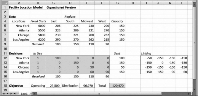
appear in column B, and the variable cost (per thousand) corresponding to each com-

bination of DC location and customer region appears in the range C5:F8.

The Decisions section of the spreadsheet contains an array for decision variables.

Column B holds the values of the y

variables. The preliminary solution shown in the

ﬁgure uses all four DC locations, so the entries in this column are all 1s. The range

C12:F15 contains a solution to the transportation subproblem that constitutes the

kernel of the model, although this solution may not be optimal. Finally, the array

I12:L15 contains the left-hand side of the linking constraints corresponding to

(7.3), expressed in the form x

2 C

. Thus, the linking constraints are satisﬁed

when each element in this array is less than or equal to zero.

Finally, the Objective section contains the evaluation of costs. The total operating

cost in cell C18 and the total distribution cost in E18 are added to generate the total cost

in G18. The model speciﬁcation is as follows.

Objective: G18 (minimize)

Variables: B12:F15

Constraints: G12:G15 ≤ G5:G8

C16:F16 ≥ C9:F9

I12:L15 ≤ 0

B12:B15 = binary

Solver ﬁnds an optimal solution that achieves a cost of $115,770 by using th e

New York, Atlanta, and Los Angeles DC locations, as shown in Figure 7.10. As

the transportation kernel shows, the optimal solution shi ps from New York to both

the East and Midwest and from Los Angeles to both the Midwest and West, while ship-

ping to the South from Atlanta. By formulating and solving an integer programming

model for its location problem, Van Horne can implement its national supply chain in

the most cost-effective fashion.

Figure 7.9. Spreadsheet model for Example 7.3.

7.4. Linking Constraints: The Facility Location Model 265