Baker K.R. Optimization Modeling with Spreadsheets

Подождите немного. Документ загружается.

As a ﬁrst cut at an optimization model, we deﬁne the following decision variables

= 1 if the city pair (i, j) occurs on the tour.

= 0 otherwise.

We can imagine an array of x

variables in an array the same size as the table of dis-

tances, although we do not need to use the variables x

on the diagonal. Next, we can

recognize that any tour must enter each city once and leave each city once. Therefore,

in order for the decisions to be feasible, only one of the entries in each row of the

decision array can equal 1 (one departure route from each city) and only one of the

entries in each column can equal 1 (one entry route into each city.) Another way to

state this requirement is that the sum along each row and the sum along each

column must be equal to 1. When we impose these constraints, we are essentially for-

mulating an assignment problem, as discussed in Chapter 3. (See Figure 3.6 for an

example.) The assignment problem requires a 1 in every row and a 1 in every

column, and its objective function is the SUMPRODUCT of the cost (distance)

array and the decision array.

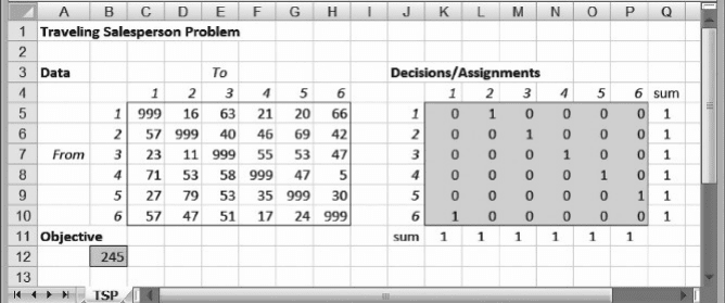
To build a spreadsheet model for the optimization problem, we ﬁrst enter the

given array of distances, as in Figure 7.15. To the right of the data we construct another

array for the decision variables x

. For each entry in the table of cleaning times, we

have a corresponding decision variable. Along the diagonal of the distance array,

we have entered arbitrarily large distances, to discourage the use of decision variables

. In the ﬁgure, we display the x-values corresponding to the cycle 1-2-3-4-5-6-1. The

objective function is the SUMPRODUCT of the data array and the decision array,

which for this sequence yields the value 245.

To ﬁnd a solution, we specify the problem as follows.

Objective: B12 (minimize)

Variables: K5:P10

Constraints: Q5:Q10 = 1

K11:P11 = 1

Figure 7.15. Distance array and decision array for Example 7.5.

276 Chapter 7 Integer Programming: Logical Constraints

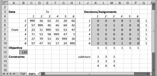
Figure 7.16 shows the result, which has an optimal objective function value of

120. Unfortunately, when we try to interpret the decision variables as a route for

the sales rep, we do not obtain a tour. Starting at city 1, the tour goes to city 5, but

then it returns to city 1. Alternatively, if we start at city 4, the tour goes to city 6

and then returns to city 4. We actually have three separate routes, called subtours,

but no tour that visits all the cities. The subtours are listed in rows 13–15 of the spread-

sheet, after Solver’s run. Evidently, the assignment problem constraints, which assure

an entry of 1 in every row and every column, are not sufﬁcient to guarantee that we can

interpret the result as a tour. We must impose additional constraints. Adding con-

straints that create a tour does not sound like it will involve linear constraints, but it

is not difﬁcult to accomplish, as we discuss next.

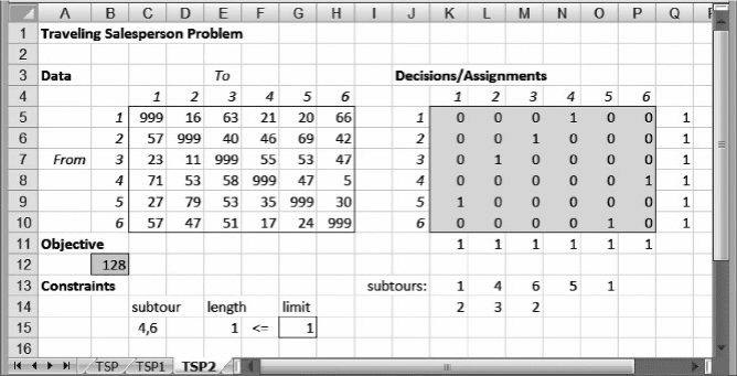
To proceed toward a solution, we have to add constraints that eliminate the

subtours we encountered. In the solution of Figure 7.17, suppose we focus on the

subtour involving cities 4 and 6. (If we can eliminate the subtour 4-6-4, that will sim-

ultaneously eliminate at least one of the other subtours. If we are fortunate, all three

subtours will be eliminated.) To prohibit the tour 4-6-4, we add the following

constraint

+ x

≤ 1

Assuming, for the moment, that the x-values are binary variables, this constraint states

that between the pair (4, 6), we can have at most one link on the tour. We place the left-

hand side of this constraint as a formula in cell E15 (under the heading “length”), and

we place the right-hand side in cell G15 (under the heading “limit”) as shown in

Figure 7.17. Now we can re-run the model with the additional constraint, hoping

that it will produce a tour.

Figure 7.16. Solution to the assignment model for Example 7.5.

7.6. Tour and Subset Constraints: The Traveling Salesperson Problem 277

This time, we specify the problem as follows.

Objective: B12 (minimize)

Variables: K5:P10

Constraints: Q5:Q10 = 1

K11:P11 = 1

E15 ≤ G15

Figure 7.17 shows the solution. The objective function increases from 120 to 128,

which is not surprising, given that we added a constraint to eliminate part of the pre-

vious solution. However, we still do not have a tour. Two subtours (1-4-6-5-1 and 2-3-

2) appear in the solution, so we must add another elimination constraint. For conven-

ience, we choose the smaller subtour and focus on 2-3-2. The appropriate constraint to

add is the following

+ x

≤ 1

We place the left-hand side in cell E16 and the right-hand side in G16, and we

again re-run the model, with the following speciﬁcation.

Objective: B12 (minimize)

Variables: K5:P10

Constraints: Q5:Q10 = 1

K11:P11 = 1

E15:E16 ≤ G15:G16

This time we obtain an objective function value of 143, and subtours of 1-2-3-1 and

4-6-5-4, as shown in Figure 7.18.

Figure 7.17. Solution for Example 7.5 with one elimination constraint.

278 Chapter 7 Integer Programming: Logical Constraints

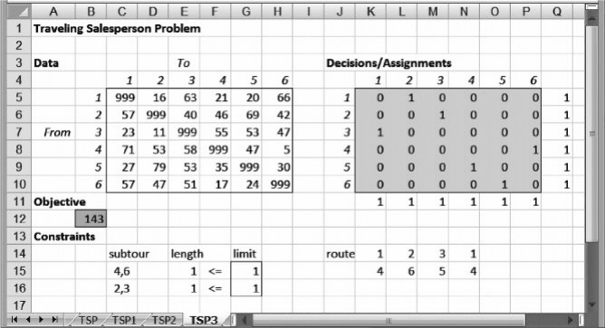
Once more, we pursue the elimination strategy. Of the two 3-city subtours,

suppose we choose to eliminate 4-6-5-4. The constraint is as follows.

+ x

≤ 2

This constraint prohibits the subtour 4-6-5-4, and while we’re at it, the subtour 4-5-6-4.

In other words, we permit at most two links on the tour from the routes involving these

three cities. The left-hand side of the constraint includes all possible city pairs from the

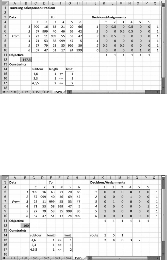
set of cities on the subtour; the right-hand side of the constraint is one less than the

number of cities in the subtour. We use cells E17 and G17 for the new constraint

and re-run the model. This time the objective function increases to 147.5, with a non-

integer solution, as shown in Figure 7.19.

Therefore, we impose the requirement that all decision variables must be binary,

specifying the problem as follows.

Objective: B12 (minimize)

Variables: K5:P10

Constraints: Q5:Q10 = 1

K11:P11 = 1

E15:E17 ≤ G15:G17

K5:P10 = binary

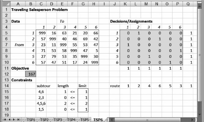
Now that we are solving an integer programming problem, we must remember to

ensure that the Integer Tolerance is zero. Then we proceed with Solver. Figure 7.20

displays the solution, which contains two subtours and achieves an objective function

of 160.

Figure 7.18. Solution for Example 7.5 with two elimination constraints.

7.6. Tour and Subset Constraints: The Traveling Salesperson Problem 279

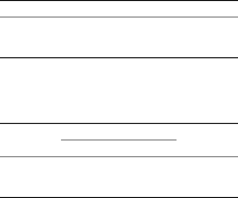
We pursue the elimination strategy one more time, eliminating the subtour 1-5-1.

Having updated the model as shown in Figure 7.21, we specify the problem as follows.

Objective: B12 (minimize)

Variables: K5:P10

Constraints: Q5:Q10 = 1

K11:P11 = 1

E15:E18 ≤ G15:G18

K5:P10 = binary

Figure 7.19. Solution for Example 7.5 with three elimination constraints.

Figure 7.20. Solution for Example 7.5 with integer requirements.

280 Chapter 7 Integer Programming: Logical Constraints

This time, the optimal solution provides a complete tour, 1-2-4-6-5-3-1, with a length

of 167, as shown in Figure 7.21. By using an integer programming approach, Douglas

Electric Cart Company can ﬁnd the color sequence that requires the minimum cleaning

time in a production cycle, thus allowing the ﬁrm to make efﬁcient use of its expensive

painting equipment.

The solution approach described here begins with an assignment model. The opti-

mal solution to the assignment model as a linear program is guaranteed to contain vari-

ables that are 0 or 1, as discussed in Chapter 3. However, the solution may or may not

represent a tour. If it does, we are fortunate, obtaining a solution to a potentially difﬁ-

cult model with a single use of linear programming. More likely, we ﬁnd that the sol-

ution contains subtours. In that case, we pursue the strategy of imposing what are

known as subtour elimination constraints. One at a time, we can add a constraint

that prohibits a subtour found in the previous optimal solution. The subtour constraint

sums the values of all the decision variables involving the city pairs in the subtour, and

requires that the sum must be less than the number of cities on the subtour.

Each time we add a subtour elimination constraint, the objective function is likely

to increase, although sometimes it may stay the same. At some stage, we may have to

impose the requirement that all variables must be binary, but that is not necessary until

we encounter a linear programming solution containing fractions. Eventually, this

iterative procedure leads to an optimal solution to the TSP.

A reasonable question to ask is why add the constraints one at a time? Of course,

when we start out, we don’t know which subtours we need to eliminate. However, we

could add constraints that eliminate all possible subtours. The problem is that this may

be a very large number of constraints. If there are n cities in the original problem, then

the number of constraints that would eliminate all subtours is 2

n –1

– n – 1. Consider

Figure 7.21. Optimal solution for Example 7.5.

7.6. Tour and Subset Constraints: The Traveling Salesperson Problem 281

that when n is 12, the number of constraints is over 2000, not to mention that we would

ﬁnd it very tedious to enter those constraints. The empirical ﬁnding seems to be that

only a very small fraction of the number of potential constraints is ever really

needed to obtain an optimal solution using the iterative procedure we have illustrated.

In our example, which contained six cities, we would have needed 25 constraints to

guarantee an optimal solution with one model, but we found that we needed only

four constraints when we implemented the one-at-a-time approach. (Most six-city pro-

blems require fewer than that.) Problems with 12, 15, or even 20 cities are usually

within the reach of spreadsheet-based solution approaches because the relatively

small number of elimination constraints actually needed is well within Solver’s

limits. The limiting factor is the time required to solve the necessary series of integer

programs en route to a ﬁnal solution.

Applications of the TSP occur frequently in manufacturing and logistics, and

some very powerful solution methods, tailored to the TSP, have been developed for

repeated use or for tackling especially large versions. The main purpose here is to illus-

trate a complex logical constraint (the tour requirement) and to demonstrate that it is

possible to apply integer programming techniques effectively for nontrivial problem

sizes. Large-scale applications require prohibitive amounts of time from Solver, and

in those cases, it would be necessary to look elsewhere for a method specialized to

the TSP.

SUMMARY

The ability to treat variables as integer-valued, and, in particular, the ability to designate certain

variables as binary, opens up a wide variety of optimization models that can be addressed with

Solver. As illustrated in Chapters 6 and 7, Solver’s branch and bound capability can handle three

broad types of models.

†

The ﬁrst type is one that resembles a linear program but with the requirement that certain

variables must be integer valued. In Solver, this requirement is added as a constraint.

†

The second type is one in which certain decisions exhibit an all-or-nothing structure,

reﬂecting actions that are indivisible. This is a role for a binary variable, which is

simply an integer-valued variable no less than zero and no greater than one. Such a vari-

able allows us to model the occurrence of yes/no choices and to use Solver, provided

that the structure of the model is linear in all other respects.

†

The third type is one in which binary variables are used to capture certain logical con-

straints in linear form. We don’t often think of logical constraints as being so closely

related to the inequalities of linear programs, so it takes some modeling practice to

appreciate how to make this connection. As the examples illustrate, binary variables

are useful in representing linking constraints for ﬁxed costs, disjunctive constraints

for sequencing problems, and tour constraints for routing problems.

The categories that rely on binary variables include a number of well known combinatorial

problems. For many of these problems, large instances can take a great deal of time to solve,

282 Chapter 7 Integer Programming: Logical Constraints

whether the solution technique is based on an integer programming formulation or some other

approach. In the case of sequencing problems or TSPs, instances with more than 20 elements

might create a substantial computational burden for Solver, even though the sizes of the

examples in this chapter do not suggest any computational difﬁculty. In moving to a larger

scale, it may be helpful to reset the Integer Tolerance parameter to a more forgiving level,

such as 5 percent, while exploring the Solver’s response time. It may also be helpful to set a

generous time limit (Max Time) on the Engine tab of the task pane, in case the computational

burden is greater than anticipated.

EXERCISES

7.1. Moore Ofﬁce Products (Revisited) Revisit the Moore Ofﬁce Products example of this

chapter, where there have been some revisions in the problem’s data. The information is

summarized below.

Family Demand Contribution Fixed cost

F1 290,000 $1.20 $60,000

F2 200,000 1.80 200,000

F3 50,000 2.30 55,000

Each product requires work on three machines. The standard productivities and capacities

are given below.

Machine

Hours per 1000 units

Hours

availableF1 F2 F3

A 3.205 3.846 7.692 1900

B 2.747 4.808 6.410 1900

C 1.923 3.205 9.615 1900

(a) Determine which products should be produced, and how much of each should be

produced, in order to maximize proﬁt contribution.

(b) Suppose the demand potential for F3 is doubled. What is the maximum proﬁt contri-

bution? How much of each product should be produced?

7.2. Selecting R&D Projects The Northeast Communications Company (NCC) is contem-

plating a research and development program encompassing eight major projects. The

company is constrained from embarking on all of the projects by the number of available

scientists (40) and the budget available for project expenses ($300,000). The following

table shows the resource requirements and the estimated proﬁt for each project.

Exercises

283

Expense Scientists Proﬁt

Project ($000) required ($000)

160736

2 110 9 82

353829

447416

592756

685661

773848

865541

(a) What is the maximum proﬁt, and which projects should be selected?

(b) Suppose that management determines that projects 2 and 5 are mutually exclusive.

What is the revised project portfolio and the revised maximum proﬁt?

ving consumer products. (These happen to be projects 5– 8.) What is the revised pro-

ject portfolio and the revised maximum proﬁt?

7.3. Vendor Allocation with Price Breaks Universal Technologies, Inc. has identiﬁed two

qualiﬁed vendors with the capability to supply some of its electronic components. For the

coming year, Universal has estimated its volume requirements for these components and

obtained price-break schedules from each vendor. (These are summarized as “all-units”

price discounts in the table below.) Universal’s engineers have also estimated each ven-

dor’s maximum capacity for producing these components, based on available information

about equipment in use and labor policies in effect. Finally, because of its limited history

with Vendor A, Universal has adopted a policy that permits no more than 60% of its total

unit purchases on these components to come from Vendor A.

Vendor A Vendor B

Unit Volume Unit Volume

Product Requirement price required price required

1 500 $225 0–250 $224 0– 300

$220 250–500 $214 300– 500

2 1000 $124 0–600 $120 0–1000

$115 600–1000 (no discount)

3 2500 $60 0 –1000 $54 0–1500

$56

∗

1000– 2000 $52 1500 –2500

$51 2000 –2500

Total capacity (units) 2500 2000

∗

For example, if 1400 units are purchased from Vendor A, they cost $56 each, for a total of $78,400.

What is the minimum-cost purchase plan for Universal?

284 Chapter 7 Integer Programming: Logical Constraints

7.4. Incremental Quantity Discount In the previous exercise, suppose that Vendor A

provides a new price-discount schedule for component 3. This one is an “incremental”

discount, as opposed to an “all-units” discount, as follows.

Unit price ¼ $60 on all units up to 1000

Unit price ¼ $56 on the next 1000 units

Unit price ¼ $51 on the next 500 units

With the change in pricing at Vendor A, what is the minimum purchasing cost for

Universal, and what is the impact on the optimal purchase plan (compared to the one

in the previous exercise)?

7.5. Plant Location The Spencer Shoe Company manufactures a line of inexpensive shoes

in one plant in Pontiac and distributes to ﬁve main distribution centers (Milwaukee,

Dayton, Cincinnati, Buffalo, and Atlanta) from which the shoes are shipped to retail

shoe stores. Distribution costs include freight, handling, and warehousing costs. To

meet increased demand, the company has decided to build at least one new plant with

a capacity of 40,000 pairs per week. Surveys have narrowed the choice to three locations,

Cincinnati, Dayton, and Atlanta. As expected, production costs would be low in the

Atlanta plant, but distribution costs are relatively high compared to the other two

locations. Other data are as follows.

To distribution

Distribution costs per pair

from

Demand

(pairs/wk)centers Pontiac Cincinnati Dayton Atlanta

Milwaukee $0.42 $0.46 $0.44 $0.48 10,000

Dayton 0.36 0.37 0.30 0.45 15,000

Cincinnati 0.41 0.30 0.37 0.43 16,000

Buffalo 0.39 0.42 0.38 0.46 19,000

Atlanta 0.50 0.43 0.45 0.27 12,000

Capacity (pairs/wk) 32,000 40,000 40,000 40,000

Production cost/pair $2.70 $2.64 $2.69 $2.62

Fixed cost /wk $7000 $4000 $6000 $7000

(a) Assume that Spencer Shoe Company will keep operating at Pontiac and build a plant

at one of the three new alternatives. Which alternative will lead to the lowest total cost,

including production, distribution, and ﬁxed costs, and what is the minimum weekly

cost?

(b) Assume that Spencer Shoe Company could start from scratch and operate any com-

bination of the four plants. Determine the plant locations that minimize total cost.

Compared to the result in part (a), how much weekly cost could be saved with the

optimal system design?

7.6. Landﬁll Location The Metropolis city council is examining four landﬁll sites as can-

didates for use in the city’s solid waste disposal network. The monthly costs per ton have

been estimated for operating at each site and for transportation to each site from the

Exercises

285