Baker K.R. Optimization Modeling with Spreadsheets
Подождите немного. Документ загружается.

begins to answer our question about local optima, it is not always an operational result.
Unfortunately, the mathematics of identifying convexity lie beyond the scope of this
book. For most practical purposes, we have a convex feasible region if we have no con-
straints at all or if we have a feasible set of linear constraints. In addition, we have a
convex or concave objective function if it is linear or if it is made up of quadratic
terms or terms involving such smooth functions as e
ax
, log(ax), and the like, with coef-
ficients that are all positive or all negative.
In some problems, we cannot tell whether the requisite conditions are satisfied, so
we cannot be sure whether the solution generated by the GRG algorithm is a global
optimum. In such cases, we may have to tolerate some ambiguity about the optimal
solution. As the previous discussion has suggested, there are two ways we can try
to build some evidence that Solver has located the global optimum. First, we can
plot a graph of the objective function and see whether it provides a confirming picture.
However, this approach is essentially limited to one- or two-variable models. A second
response is to re-run Solver starting from several different initial points to see whether
the same optimal solution occurs. However, there is no theory to tell us how many such
runs to make, how to select the initial points advantageously, or how to guarantee that
a global optimum has been found.
In a nonlinear problem, if we run Solver only once, we may have to be lucky to
obtain the global optimum, unless we know something about the problem’s special
features. To help convince ourselves that Solver has found the global optimum, we
might try rerunning from different starting points to see whether the same solution
occurs. Even then, we can’t be too casual about selecting those starting points; in
the quantity discount example, starting points between 216 and 499 lead to the
same suboptimal result. In a complicated, multidimensional problem, we might
have to test many starting points to give us a reasonable chance of finding a global opti-
mum. However, it was just this type of effort that we were trying to avoid by using
Solver in the first place.
Solver contains a MultiStart option that automates the process of re-running with
different starting values of the decision variables. This option can be found on the
Engine tab of the task pane, in the Global Optimization section. (The default value
for this option is False.) When using this option, it is necessary to specify upper
and lower bounds for all decision variables. The nonnegativity requirement, assuming
it applies, can serve as a lower bound, but the user must supply an upper bound if none
is contained in the original formulation.
Thus, when we use Solver, we must consider whether the algorithm we use,
applied to the optimization problem we have posed, is a reliable algorithm. By that,
we mean the algorithm is guaranteed to find a global optimum whenever one exists.
The simplex method, applied to linear programs, is always reliable. The GRG algor-
ithm, applied to nonlinear programs, is reliable only in special circumstances.
Because the GRG algorithm is the default choice of a solver, it is tempting to use it
when solving linear programming problems as well as nonlinear programming pro-
blems. A problem containing a linear objective function and linear constraints quali-
fies as one of the problem types in which the nonlinear solver is reliable. However, two
possible shortcomings exist in solving linear problems. First, the GRG algorithm may
306
Chapter 8 Nonlinear Programming

not be able to locate a feasible solution if the initial values of the decision cells are
infeasible. Sometimes, it may be difficult to construct a solution that satisfies all con-
straints, just for the purposes of initiating the steepest ascent method used in the non-
linear solver. In some cases, the nonlinear solver will report that it is unable to find a
feasible solution, even when one exists. By contrast, the linear solver is always able to
locate a feasible solution when one exists. A second reason for preferring the linear
solver for linear problems relates to numerical aspects of the model. In some cases,
the nonlinear solver may be unable to find an optimal solution without requiring
the Automatic Scaling option, whereas the linear solver would not encounter such a
problem.
When it comes to problems with integer constraints on some of the variables,
Solver augments its basic solution algorithm with a branch-and-bound procedure,
as described in Chapter 6. The branch-and-bound method involves solving a series
of relaxed problems—that is, problems like the original but with integer constraints
removed. When the branch-and-bound procedure is applied to a linear model, in
which the simplex method is reliable, we can be sure that the search ultimately locates
an optimum. However, when the branch-and-bound procedure involves a series of
nonlinear models, we cannot be sure that the relaxed problems are solved to optimal-
ity. Therefore, the search may terminate with a suboptimal solution. For that reason,
we should avoid using Solver on nonlinear integer programming problems, although
the software permits us to use this combination.
8.3. TWO-VARIABLE MODELS
When we move from one decision variable to two, the analysis remains manageable.
To check Solver’s result, we can plot the outcomes of a two-dimensional grid search,
based on using Excel’s Data Table tool. We can also investigate the objective function
behavior one variable at a time. Although such investigations are not foolproof in two
dimensions, they are likely to be quite helpful. The examples that follow illustrate
some of Solver’s applications.
8.3.1. Curve Fitting
A common problem is to find a smooth function to fit observed data points. A more
sophisticated, statistically-oriented version of this problem is known as regression,
but here we take only the first step. Consider the Fitzpatrick Fuel Supply Company
as an example.
EXAMPLE 8.3
The Fitzpatrick Fuel Supply Company
The Fitzpatrick Fuel Supply Company, which services residential propane gas tanks, would like
to build a model that describes how gas consumption varies with outdoor temperature
conditions. Knowledge of such a function would help Fitzpatrick in estimating the short-term
8.3. Two-Variable Models
307

demand for propane. A sample of 12 observations was made at customers’ houses on different
days, and the following observations of degree-days and gas consumption were recorded.
Degree Gas
Day days consumption
110 51
211 63
313 89
4 15 123
5 19 146
6 22 157
7 24 141
8 25 169
9 25 172
10 28 163
11 30 178
12 32 176
(A degree day is one full day at a temperature 1 degree lower than the level at which heating is
needed—usually 688.) For each day in the table, the number of degree days represents an aver-
age over the day. As a first cut at the estimation problem, Fitzpatrick’s operations manager would
like to fit a linear model to the observed data.
B
The proposed linear model takes the form y ¼ a þ bx, where y is the gas con-
sumption in cubic feet and x is the number of degree days. The problem is to find
the best values of a and b for the model. Standard practice in this type of problem
is to minimize the sum of squared deviations between the model and the observations.
The curve-fitting technique proceeds by calculating, for each of the observations,
the difference between the model value and the observed value. If the k
th
observation
is represented as (x
k
, y
k
), then the difference between the model and the k
th
observation
can be written as follows.
Difference ¼ Model value Observed value
d
k
(a, b) ¼ (a þ bx
k
) y
k
A measure of how good a fit the model achieves is the sum of squared differences
(between model value and observation value) or
f (a, b) ¼
X
k
[d
k
(a, b)]
2
A small sum indicates that the fit is quite good, and our objective in this case is to mini-
mize the sum of squared deviations. In this formulation, the model parameters a and b
are the decision variables, and the objective is to minimize f(a, b). Figure 8.8 displays a
spreadsheet for the curve-fitting problem. The first module contains the decision vari-
ables (the model parameters a and b) in cells E3 and E4, and the second module con-
tains a single-cell objective in E5. The third module contains the data along with
308
Chapter 8 Nonlinear Programming
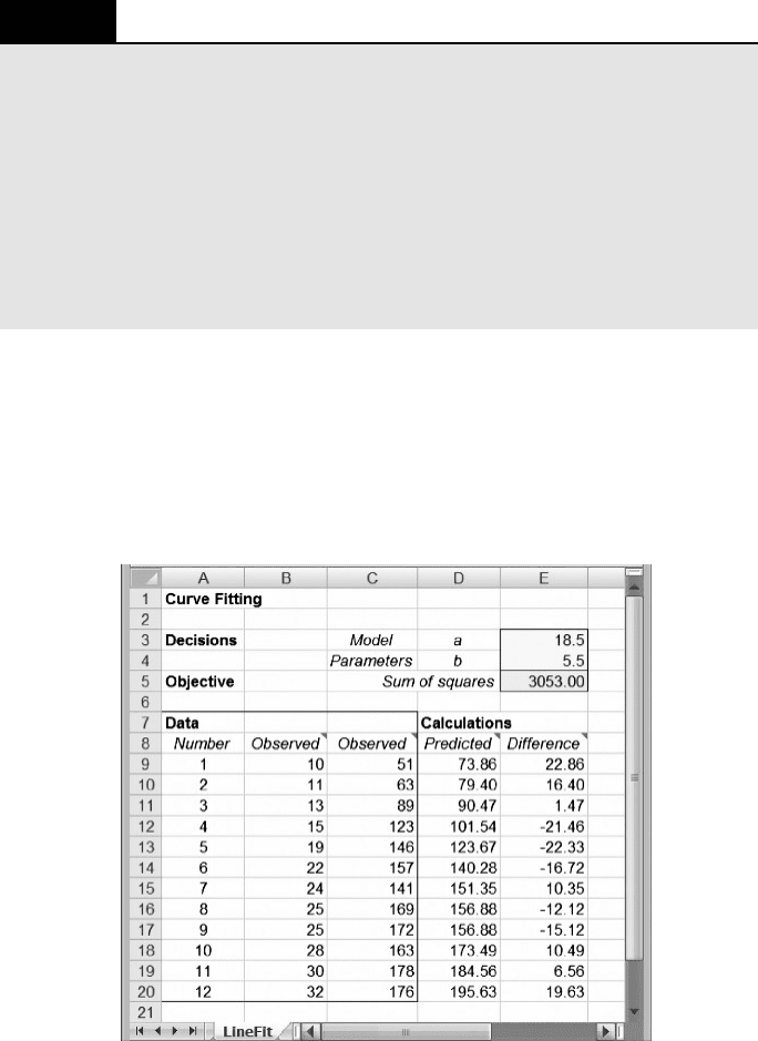
calculations of the predicted values and their differences from observed values. The
sum of squared differences is calculated from these differences using the SUMSQ
function.
We specify the problem as follows.
Objective: E5 (minimize)
Variable: E3:E4
The solution, as displayed in Figure 8.9, is the pair (18.5, 5.5), for which the sum of
squared deviations is approximately 3053. This means that the best predictive model
BOX 8.1
Excel Mini-Lesson: The SUMSQ Function
The SUMSQ function in Excel calculates the sum of squared values from a list of numbers.
The numbers can be supplied as arguments to the function, or the argument(s) can be cell
references. The form of the function is the following
SUMSQ(Number1, Number2, ...) or SUMSQ(Array)
In cell E5 of Figure 8.9, the function
=SUMSQ(E9 :E20) squares each of the 12 elements
in the Difference column and then adds the squares. If we were to enter the values 10 and 6
in cells E3 and E4, respectively, the total would be 3208. Because the need to compute a
sum of squares is encountered frequently, Excel provides this function to streamline the
calculation.
Figure 8.9. Spreadsheet for Example 8.3.
8.3. Two-Variable Models 309

for the 10 observations is the line y ¼ 18.5 þ 5.5x. Using this simple function,
Fitzpatrick Fuel Supply can make reasonable predictions of propane consumption
as the daily temperature varies. With this capability, along with short-term forecasts
of daily temperatures, Fitzpatrick can predict future demand and thereby position its
inventories appropriately.
The curve-fitting model can easily be extended to functions other than the linear
model (or to functions with more than two parameters). For example, we might guess
that a better model for consumption would be the power model y ¼ ax
b
. If we had
reason to believe that this model contained better predictive power, we could revise
the spreadsheet to test it. We simply have to take the linear model out of cells
D9 : D20 and substitute the power model. Re-running Solver with this change in the
model yields a minimum sum of squared deviations equal to approximately 2743,
which is a lower figure than can be achieved by any linear model. The best fit in
the power family is the function y ¼ 11.5x
0.81
. Although there may well be structural
reasons to prefer a model with diminishing returns (because the fuel is less efficient
when used intermittently, at low x-values), the optimization criterion also leads us
to the power model as a preferable choice in terms of minimizing the sum of squared
deviations.
The curve-fitting model with a linear predictor and a sum-of-squares criterion
has a convex objective function. This structure tells us that the optimization is
straightforward, and we don’t have to worry about local optima. For the sum-of-
squares criterion, the local optimum found by Solver will always be the global opti-
mum. A more challenging problem would arise if some other criterion were used. For
example, had the criterion been to minimize the sum of absolute deviations, the
optimization problem would have been more difficult. (We investigate this variation
in Chapter 9.)
8.3.2. Two-dimensional Location
A common problem is to find a location for a facility that serves many customer sites.
In Chapter 7, we encountered the discrete version of the facility location problem,
which involves a specific set of possible locations. However, a first cut at a location
problem might be helpful before we know the details of possible locations. In such
cases we can approach the problem from a continuous perspective. Most often, the
continuous location problem arises in two dimensions, as in the case of Merrill
Sporting Goods.
EXAMPLE 8.4
Merrill Sporting Goods
Merrill Sporting Goods has decided to build a centrally located warehouse as part of its distri-
bution system. The company manufactures several types of sports equipment, stocks them at the
factory warehouse, and delivers to a variety of retail sites. Having outgrown its current ware-
house and wanting to take advantage of new warehousing equipment, the firm has decided to
build at a fresh location. To define a central location, their ten retail sites are first mapped on
310 Chapter 8 Nonlinear Programming

a two-dimensional grid, so that the coordinates (x
k
, y
k
) can be associated with each site. These
values are as follows.
Site (k) x
k
y
k
1929
2550
32668
43979
54154
63859
7636
85258
98176
10 95 93
A good location is one that is “close” to all sites. To make this concept operational, Merrill’s
distribution manager suggests that the objective should be to minimize the sum of the distances
between the warehouse and the various sites. Using this measure as a criterion, the distribution
manager wishes to find the optimal location for the warehouse.
B
To begin the analysis, we represent the location of the warehouse by the coordi-
nates (x, y). The straight-line distance in two dimensions between the warehouse and
the k
th
site (also known as the Euclidean distance) is given by
D
k
(x, y) ¼ (x x
k
)
2
þ ( y y
k
)
2
1=2
Based on this definition, we can express Merrill’s objective function as follows
f (x, y) ¼
X
10
k¼1
D
k
(x, y)
The problem is to find the decision variables (x, y) that minimize the total distance
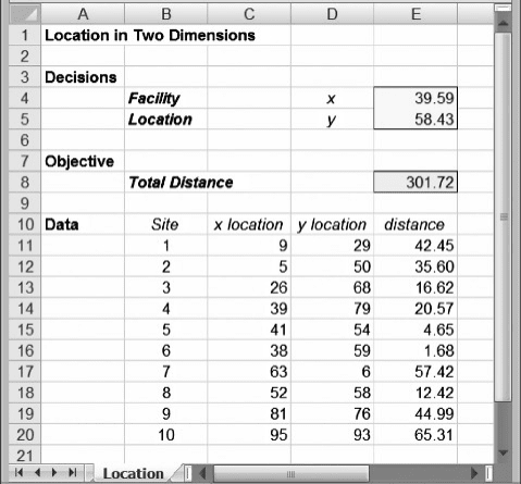
function f(x, y). The problem has no explicit constraints. Figure 8.10 shows a spread-
sheet for the problem, where the coordinates of the warehouse location appear in cells
E4 and E5, and the total distance objective appears in cell E8. The detailed data appear
in the last module.
We specify the problem as follows
Objective: E8 (minimize)
Variable: E4:E5
The solution, as displayed in Figure 8.10, is the location (39.59, 58.43), for which the
objective function reaches a minimum of approximately 301.72. The conclusion for
Merrill Sporting Goods is that the map location corresponding to approximately
(40, 58) represents the central location they seek.
8.3. Two-Variable Models 311
We might wonder whether this figure represents a global optimum. As discussed
earlier, we can re-run Solver from a variety of starting solutions. Starting with a variety
of different solutions, we find that Solver always leads us to the same optimal solution
of about (40, 58). Plots of the objective function as we vary x or y separately suggest a
similar story. Thus, we have at least some informal evidence that our solution is a
global optimum. (Because this is a two-variable optimization model, we could use
the Data Table tool to confirm this result.)
8.4. NONLINEAR MODELS WITH CONSTRAINTS
In terms of building spreadsheet models, it is no more difficult to add a constraint in a
nonlinear program than it is to add a constraint in a linear program. When using Solver,
the steps are identical. Perhaps the only important difference lies in what we might
expect as a result.
The key difference between linear and nonlinear models can be illustrated with
graphs of a one-dimensional problem. Figure 8.11 shows both the linear and nonlinear
cases. In the first graph, the objective is linear, in the form f(x) ¼ cx. The decision vari-
able x must satisfy the constraints x a and x b. It is easy to see that the optimal
value of the objective function must occur when the decision variable lies at one of
the constraint boundaries. In a maximization problem, the optimum would be x ¼
b; in a minimization problem, the optimum would be x ¼ a. (The conclusions
would be similar if the linear objective had a negative slope rather than a positive one.)
Figure 8.10. Spreadsheet for Example 8.4.
312 Chapter 8 Nonlinear Programming
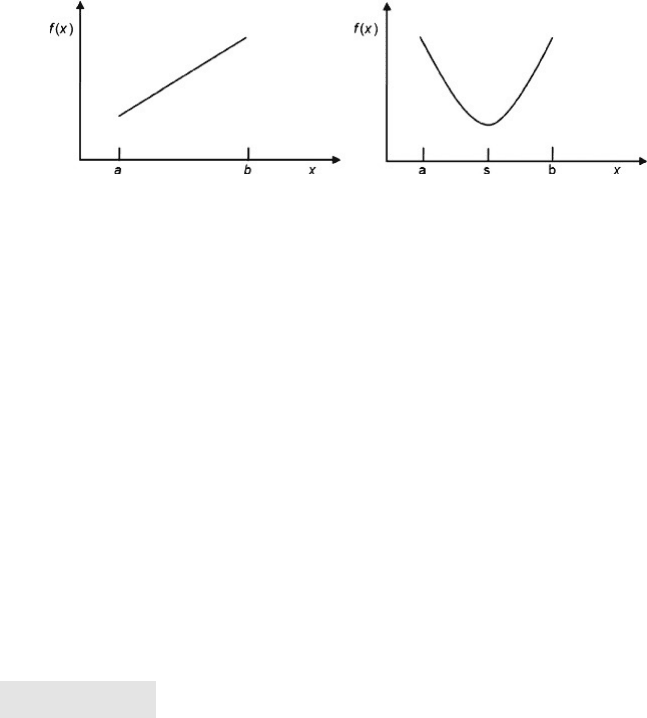
In the second graph, the objective is nonlinear, in the form f (x) ¼ (x 2 s)
2
, and
the same two constraints apply. Assuming that the parameter s lies between a and
b, the minimum value of f(x) occurs at x ¼ s, and neither of the constraints is binding.
On the other hand, the maximum value of f(x) does lie at one of the constraint
boundaries.
This graphical example shows that we should always expect at least one constraint
to be binding for a linear objective, but that may not be so for a nonlinear objective. In
the nonlinear case, the mathematical behavior of the objective function may lead to an
optimal decision for which no constraints are binding.
8.4.1. A Pricing Example
When a problem contains both price and quantity decisions, it is likely that a nonlinear
programming model will result. The nonlinearity derives from the fact that profit on a
given product is equal to (Price 2 Cost) Volume, and Price depends on Volume.
Consider the situation at Nells Furniture Company.
EXAMPLE 8.5
Nells Furniture Company
Nells Furniture Company (NFC) sells two main products, sofas and dining tables. Based on the
last few years of experience in the sales region, the marketing department has estimated demand
curves relating the price and demand volume for each product. For sofas, the relationship is
p
1
¼ 220 0:4x
1
where p
1
and x
1
are the price and volume, respectively. For tables, the price –volume relation-
ship is
p
2
¼ 180 0:2x
2
The variable costs are $60 per unit for the sofas and $45 per unit for the tables. Each item is
assembled on site and then inspected carefully. The inspection usually involves some rework
and touch-up. There are 800 hours available in the assembly department and 500 in the inspec-
tion department. Sofas require 2 hours assembly time and 2 hours inspection time. Tables
require 3 hours assembly time and 1 hour inspection time. The management at NFC wants to
maximize profit under these conditions. B
Figure 8.11. Linear and nonlinear objective functions.
8.4. Nonlinear Models with Constraints 313
Taking the volumes x
1
and x
2
as decision variables, we first write the objective func-
tion in terms of these variables by substituting for p
1
and p
2
Profit ¼ ( p
1
60)x
1
þ ( p
2
45)x
2
¼ (160 0:4x
1
)x
1
þ (135 0:2x
2
)x
2
The constraints in the problem are linear constraints
2x
1
þ 3x
2
800 (assembly)
2x
1
þ x
2
500 (inspection)
The problem becomes one of maximizing the nonlinear profit function, subject to two
linear constraints on production resources.
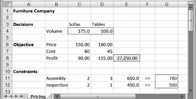
Figure 8.12 shows a spreadsheet model for the problem. The three modules in the
spreadsheet correspond to decision variables, objective function, and constraints. In
the objective function module, we list the unit price, unit cost, and unit profit explicitly.
The unit price of sofas in cell C6 is given by the formula relating sofa price and sofa
volume, and similarly for the unit price of tables in cell D6. This layout allows us to
express the total profit using a SUMPRODUCT formula, although it is not a linear
function. Finally, the constraints are linear, so their structure follows the form we
have seen in earlier chapters for linear programs.
We specify the problem as follows
Objective: E8 (maximize)
Variables: C4:D4
Constraints: E11:E12 G11:G12
Solver returns the optimal decisions as approximately 144 sofas and 170 tables. The
corresponding prices are $162.27 and $145.91, and the optimal profit is about
$31,960. Although we formulated the model using volumes as decision variables, it
Figure 8.12. Spreadsheet for Example 8.5.
314 Chapter 8 Nonlinear Programming
would probably be the case in this type of a setting that the focus would be on
prices. As the model indicates, optimal prices are approximately $162 and $146 for
sofas and tables, respectively. By solving this optimization problem, NFC has an
idea how to set prices in the face of a price-sensitive customer market.
8.4.2. Sensitivity Analysis for Nonlinear Programs
In Chapter 4, we described two software-based procedures for sensitivity analysis,
Parameter Sensitivity and the Sensitivity Report. For nonlinear programs, the use of
the Parameter Sensitivity tool is essentially the same as it is for linear programs.
However, the Sensitivity Report is a little different, and we describe it here.
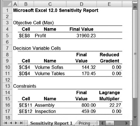
Returning to the example of the previous section, suppose we optimize the NFC
example and then create the Sensitivity Report. Solver provides the report shown in
Figure 8.13. As in the case of linear programs, there are three parts to the report, relat-
ing to objective function, decision variables, and constraints. For decision variables,
the report lists the optimal value for each variable (which, of course, repeats infor-
mation on the worksheet itself) along with the reduced gradient. This value, like
the reduced cost in linear programs, is zero if the variable does not lie at its bound.
For constraints, the report lists the optimal value for each left-hand side
(again, duplicating information in the spreadsheet) along with the Lagrange multi-
plier. This value is essentially a shadow price. When the constraint is not binding, the
shadow price is zero; otherwise, the Lagrange multiplier provides us with the instan-
taneous rate of change in the objective function as the constraint constant changes.
Figure 8.13. Sensitivity report for Example 8.5.
8.4. Nonlinear Models with Constraints 315