Baker K.R. Optimization Modeling with Spreadsheets
Подождите немного. Документ загружается.


For example, suppose we vary the number of assembly hours in the NFC model
and reoptimize. The table below, obtained from the Parameter Sensitivity tool, sum-
marizes the results for values above and below the given value of 800 hours.
Assembly hours Optimal profit Rate of change
750 30,801 –
760 31,040 23.91
770 31,276 23.55
780 31,508 23.18
790 31,736 22.82
800 31,960 22.45
810 32,181 22.09
820 32,398 21.73
Thus, when the number of assembly hours changes from 770 to 780, the optimal
profit improves by $231.82 (¼ 31,507.50 – 31,275.68), or $23.18 per additional
assembly hour over this interval. From the table, we can see that the value of an
additional hour of assembly time varies depending on the number of assembly
hours in the model, dropping from nearly $24 to under $22 over the range shown.
The rate of change in the table is calculated from changes in the optimal profit on
a grid of size 10. If we reduced the grid to size five or size one, we would see that
rate change more gradually, row to row. The entry for 800 assembly hours would
change from $22.45 on the size 10 grid to $22.36 on the size five grid, and to
$22.29 on the size one grid. We can imagine continuing this process to ever finer
grids. As we do so, the incremental value of assembly hours declines, and the rate
of change at 800 gets ever closer to a limiting value of $22.27. This limiting value
corresponds to the Lagrange multiplier.
The Sensitivity Report provides the shadow price for linear programs and the
Lagrange multiplier for nonlinear programs. Their values are zero when the constraint
is not binding; and when the constraint is binding, their values give the incremental
value of the scarce resource. In the typical linear program, however, this incremental
value stays constant for some amount of increase or decrease in the constraint con-
stant. In the typical nonlinear program, as illustrated here, this incremental value is
always changing with the constraint constant. The Lagrange multiplier represents only
the instantaneous rate of change. For that reason, no ranging information, such as the
allowable increase or decrease reported in the linear model, would be appropriate.
8.4.3. The Portfolio Optimization Model
A portfolio is a collection of assets. In a stock portfolio, the investor chooses the
stocks, and the dollar value of each, to hold in the portfolio at the start of an investment
period. Over this period, the values of the stocks may change. At the end of the period,
performance can be measured by the total value of the portfolio. For a given size (or
316
Chapter 8 Nonlinear Programming

dollar value) of the portfolio, the key decision is how to allocate the portfolio among
its constituent stocks.
A stock portfolio has two important projected measures: return and risk. Return is
the percentage growth in the value of the portfolio. Risk is the variability associated
with the returns on the stocks in the portfolio. The information on which stocks are
evaluated is a series of historical returns, typically compiled on a monthly basis.
This history provides an empirical distribution of a stock’s return performance. For
stock k in the portfolio, this return distribution can be summarized by a mean (r
k
)
and a standard deviation (s
k
).
EXAMPLE 8.6
Counseling Ms Downey
Suppose we are providing investment advice to Ms Downey, who has a nest egg to invest and
some very clear ideas about her preferred stocks. In fact, she has identified stocks in five different
industries that she believes would constitute a good portfolio. The performance of the five stocks
in two recent years is summarized by the following data.
Stock Mean St. dev.
National Computer 0.0209 0.0981
National Chemical 0.0121 0.0603
National Power 0.0069 0.0364
National Auto 0.0226 0.0830
National
Electronics
0.0134 0.0499
Ms Downey does not, however, know how to allocate her investment among these five
stocks. National Computer Company and National Auto Company stocks have achieved the
best average returns in the two-year period, but they also have relatively high volatility, as
measured by their standard deviations. National Power Company is the least volatile, but it
also has the lowest average return. Ms Downey wishes to navigate between these different
extremes. Our task is to organize this quantitative information so that we can help her make
the allocation decision. B
Figure 8.14 shows a worksheet containing the monthly returns for Ms Downey’s five
stocks over the last two years. The data can be found in columns I through N. The mean
returns are calculated using the AVERAGE function in cells B4:F4, and the standard
deviations are calculated using the STDEV function in cells B5:F5.
Next, the task is to combine the individual stock behaviors into a summary for the
portfolio as a whole—that is, a calculation of the mean and variance. For the portfolio
mean, we use a weighted average of individual stock returns. Thus, if we allocate a
proportion p
k
of our portfolio to stock k, then the return on the portfolio is the weighted
average
R ¼
X
k
p
k
r
k
8.4. Nonlinear Models with Constraints 317
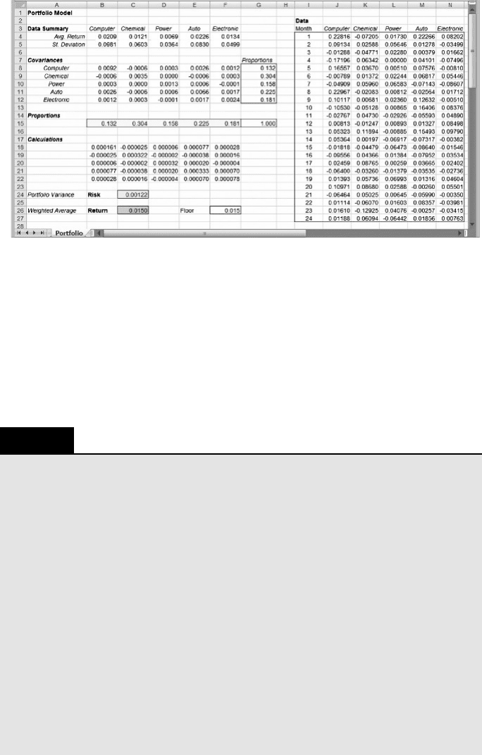
This calculation lends itself to the SUMPRODUCT formula and appears in the
worksheet in cell C26. The proportions themselves, highlighted as decision variables,
appear in cells B15:F15, with their sum in cell G15.
For the portfolio variance, we use a standard statistical formula for the variance of
a sum. For this purpose, we must know the covariance
s
kj
between every pair of stocks
(k, j). The covariance values are calculated from the historical data with Excel’s
COVAR function. These figures appear in the spreadsheet in cells B8:F12.
Figure 8.14. Spreadsheet model for Example 8.6.
BOX 8.2
Excel Mini-Lesson: The COVAR Function
The COVAR function in Excel calculates the covariance between two equal-sized sets of
numbers representing observations of two variables. The covariance measures the extent to
which one variable tends to rise or fall with increases and decreases in the other variable. If
the two variables rise and fall in unison, their covariance is large and positive. If the two
variables move in opposite directions, their covariance is negative. If the two variables
move independently, their covariance is close to zero. The basic form of the function is
COVAR(Array1, Array2)
†
Array1 references the observations of the first variable.
†
Array2 references the observations of the second variable.
The arrays must be of the same size.
In cell C11 of Figure 8.14, the function
=COVAR($M4:$M27,$K4:$K27) finds the
covariance between the returns of National Chemical Company and those of National
Auto Company. In this case, the function generates the value –0.0006. The fact that it is
a small number in absolute value indicates that the two sets of returns are nearly indepen-
dent; the fact that it is negative indicates that there is a slight tendency for National Auto’s
returns to go up when National Chemical’s returns go down, and vice versa.
318 Chapter 8 Nonlinear Programming
The formula for the portfolio variance is
V ¼
X
k
X
j
p
k
s
kj
p
j
This formula sometimes appears in statistics books in a different but equivalent form.
From this form, however, it is not difficult to make the calculation in Excel. The value
of p
k
s
kj
p
j
is computed as the (k, j)th element of the array in cells B18:F22. (For this
purpose, it is convenient to replicate the proportions from row 15 in cells G8:G12.)
Then the elements of this array are summed in cell C24. As a result, the risk measure
V appears in cell C24, and the return measure R appears in C26.
The portfolio optimization problem is to choose the investment proportions to
minimize risk subject to a floor (lower bound) on the return. That is, we want to mini-
mize V subject to a minimum value of R, with the p-values as the decision variables. A
value for the lower bound appears in cell F26. We specify the model as follows.
Objective: C24 (minimize)
Variables: B15:F15
Constraints: C26 F26
G15 ¼ 1
For a return floor of 1.5 percent, Solver returns the solution shown in Figure 8.14.
All five stocks appear in the optimal portfolio, with allocations ranging from 30 per-
cent of the portfolio in National Chemical to 13 percent of the portfolio in National
Computer.
For this model, the spreadsheet layout is a little different from the others we have
examined, mainly due to the close relationship between the historical data and the
elements of the analysis. The spreadsheet, as constructed, could easily be adapted
to the optimization of any five-stock portfolio. All that is needed is the set of returns
data, to be placed in the data section of the spreadsheet. For a data collection period of
longer than 24 periods, the formulas for average, standard deviation, and covariance
would have to be adjusted. The Calculations section separates the decision variables
from the objective function, but the logic of the computations flows from
Proportions to Calculations to Risk and Return.
In principle, two modeling approaches are possible in portfolio optimization.
Minimize portfolio risk, subject to a floor on the return
or
Maximize portfolio return, subject to a ceiling on the level of risk
The former structure is usually adopted, because it involves a convex objective and
linear constraints, a case for which the GRG algorithm is reliable.
Beyond a single optimization of the portfolio model, investors are usually inter-
ested in the tradeoff between risk and return. If we minimize risk subject to a floor on
the return, we can repeat the optimization for several values of the floor. This process
traces out points along the so-called efficient frontier, which plots the best risk achiev-
able for any desired level of return. A complementary approach is available if we maxi-
mize return subject to a ceiling on risk. Results from the Optimization Sensitivity tool
8.4. Nonlinear Models with Constraints 319
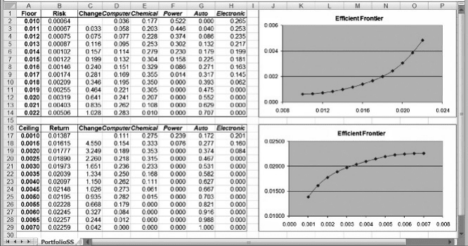
for these two approaches, along with summary plots, are shown in Figure 8.15. Both
plots describe the same risk-return trade-off; they just happen to take slightly different
forms. By exploring Ms. Downey’s preferences as they play out in these graphs, we
can make a more persuasive recommendation on how her investment funds should
be allocated.
8.5. LINEARIZATIONS
As discussed earlier, the linear solver is a reliable procedure when we apply it to solve
a linear programming problem, but the GRG algorithm is not reliable in general for a
nonlinear programming problem. For that reason, and especially when our model con-
tains integer variables, we always prefer to solve a linear model rather than a nonlinear
model. Some problems that are formulated naturally with nonlinear functions can be
reformulated as linear programs. Two examples of these transformations, or lineariza-
tions, are presented in this section.
Our purpose here is to show how to convert certain nonlinear forms to linear
forms permitting us to construct a linear model before invoking Solver. It’s important
to know that RSP contains an option that can automate these linearizations, but with
very little transparency. As a first step, it is helpful to turn off these automated pro-
cedures, and to do so, we set the Nonsmooth Model Transformation option to
Never on the Platform tab of the task pane. The default option is Automatic, but we
will assume the user has selected Never instead.
8.5.1. Linearizing the Maximum
Suppose our objective function is the maximum of several expressions involving
decision variables, such as max
k
{
P
j
a
kj
x
j
}. Presumably, we would encounter this
Figure 8.15. The efficient frontier in Example 8.6.
320 Chapter 8 Nonlinear Programming
kind of objective in a minimization problem. The natural way to represent this criterion
in a spreadsheet model would be to use Excel’s MAX function in the objective, or in
cells referenced in the objective. If we were to invoke the linear solver, we may
encounter an error message stating that our model does not satisfy its linearity require-
ments (because the MAX function is not linear). If we invoke the nonlinear solver, we
may get a solution, but we cannot be sure that it is a global optimum.
To improve our results, we can convert to a linear form by introducing a variable y
that plays the role of the maximum. Then we add definitional constraints of the form
y
X
j
a
kj
x
j
(8:1)
With the variable y as the objective function to be minimized, we have a linear model,
so we can use the linear solver. As an example, consider the situation at the Armstrong
Advertising Agency.
EXAMPLE 8.7
Armstrong Advertising Agency
The Armstrong Advertising Agency has several publishing projects that are ready for pro-
duction. Four departments are capable of implementing these projects, and the agency wants
to distribute the work among departments as evenly as possible.
Each of the projects will take a certain number of days. The following table shows the work-
load in each project, as estimated by the sales manager.
Project 1234567 8
Days 10 21 32 53 65 77 89 100
Distributing work “as evenly as possible” is not a precise description of an objective function; it
tells us only what an ideal solution would look like. In this problem, with 447 days’ worth of
work, an ideal solution would allocate 111.75 days to each department. However, because indi-
vidual projects cannot be split, we know that an ideal solution is impossible. The substantive
question for determining an objective function is how to measure a nonideal solution. At
Armstrong, the notion of distributing work evenly derives from a goal of fairness. Therefore,
the consensus is that the best solution is one that minimizes the largest amount of work assigned
to any of the departments.
B
A natural algebraic formulation of the problem is straightforward. Let a
j
represent the
time for project j, and define the following binary decision variables.
x
kj
¼ 1, if project j is assigned to department k
¼ 0, otherwise
With this notation, the optimization model is as follows
Minimize z ¼ max
k
X
j
a
j
x
kj
()
subject to
X
k
x
kj
¼ 1 for j ¼ 1, 2, ...,8
8.5. Linearizations 321
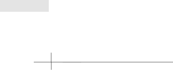
A spreadsheet model for assigning the projects to the four departments is shown in
Figure 8.16. The times required for the projects are entered in cells B5:I5. Binary vari-
ables assigning each project to a department are displayed in the array B7:I10. The row
below this array contains the sum of the decision variables in each column—the sum
over all departments. The column to the right of this array shows the total number of
days assigned to each department, and the maximum of these values, computed in cell
J4 with the formula
¼ MAX(J7:J10), serves as the objective function.
We specify the problem as follows
Objective: J4 (minimize)
Variables: B7:I10
Constraints: B11:I11 ¼ 1
B7:I10 ¼ binary
Normally, the linear solver does not run on this model because of the presence of the
MAX function, which is technically a nonsmooth function. In the output window of
the task pane, Solver’s error message appears when an attempt is made to use the linear
solver.
The linearity conditions required by
this Solver engine are not satisfied.
In contrast, the nonlinear solver does run, but it may not find an optimal solution
because the model contains binary variables as well as nonlinearity. However, a lin-
earization is possible. We can introduce a new variable y to represent the largest of
the departmental workloads, as in (8.1). This variable is displayed in cell J4 and treated
like the other decision variable cells, as shown in Figure 8.17. But this cell is special,
because it is also the value of the objective function. In addition to the constraints
already formulated, we need to add constraints requiring y to be at least as large as
the total number of days assigned to each department.
Figure 8.16. Spreadsheet model for Example 8.7.
322 Chapter 8 Nonlinear Programming
We specify the problem as follows
Objective: J4 (minimize)
Variables: B7:I10
J4
Constraints: B11:I11 ¼ 1
B7:I10 ¼ binary
J7:J10 J4
The last set of constraints is unconventional because the right-hand side appears to be
just one cell, while the left-hand side references an array of four cells. However, Solver
interprets the meaning correctly. Alternatively, the constraint could be expressed in a
more standard fashion.
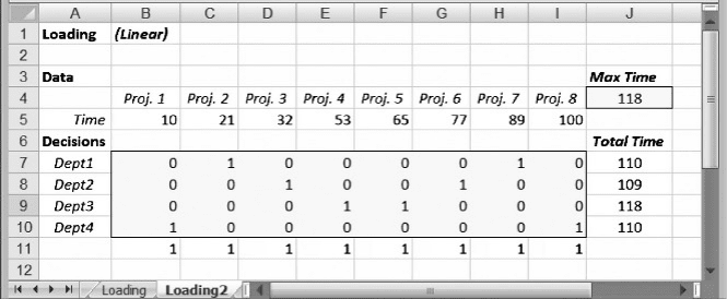
The linear solver returns the solution shown in Figure 8.17 quickly and reliably.
The workloads at Armstrong will be 109, 110, 110, and 118 days, so that the entire set
of projects will take 118 days to complete. By using the linearized model, Armstrong
can be sure that the work is distributed in the fairest way, at least when fairness is
defined to mean minimizing the maximum workload.
As this example demonstrates, the transformation of the MAX function to a linear
form is not difficult, but Solver offers the capability of making the transformation auto-
matically. This transformation would be initiated if we set the Nonsmooth Model
Transformation option to Automatic (or to Always) on the Platform tab in the task
pane. This option is convenient because we can set up the model in an intuitive
fashion, even if it does not satisfy the linearity requirement, and Solver can compen-
sate by performing the necessary transformation. However, the transformation actually
implemented by Solver is not visible to the user, so it’s not possible to know precisely
how the model is transformed. For example, in the case of Example 8.7, the original
model contains 32 variables and 8 constraints. Our transformation, shown in
Figure 8.17, uses 33 variables and 12 constraints. Solver’s automatic transformation
Figure 8.17. Optimal solution for Example 8.7.
8.5. Linearizations 323
uses 38 variables and 21 constraints, as reported in the Current Problem section of
the Engine tab. (Solver’s summary counts the objective function as a separate con-
straint.) Thus, the details of the automatic transformation may be a bit different than
the manual transformation, but the details of the automatic transformation are not
made available to the user.
8.5.2. Linearizing the Absolute Value
Suppose our objective function contains terms involving absolute value expressions,
such as j
P
j
a
kj
x
j
j. The natural way to build a spreadsheet model would be to use
Excel’s ABS function in the objective function, or in cells referenced by the objective
function. If we were to invoke the linear solver, we may see an error message,
either stating that our model does not satisfy the linearity requirements (because the
ABS function is nonsmooth) or stating that the model is unbounded. If we invoke
the nonlinear solver, we may get a solution, but we cannot be sure that it is a global
optimum.
To tackle this problem, we can define a pair of auxiliary variables, u
k
and v
k
,to
account for the difference between
P
j
a
kj
x
j
and zero. Then we include constraints of
the following form
X
j
a
kj
x
j
þ u
k
v
k
¼ 0(8:2)
In this linear formulation, two cases arise.
If
P
j
a
kj
x
j
0, then v
k
¼ 0 and u
k
measures the negative difference (if any).
If
P
j
a
kj
x
j
0, then u
k
¼ 0 and v
k
measures the positive difference (if any).
In either case, the value of (u
k
þ v
k
) measures the absolute value of the difference
between
P
j
a
kj
x
j
and zero. In the objective function, we can then use (u
k
þ v
k
)in
place of the original absolute value expression.
As an example, we return to the situation at the Armstrong Advertising Agency in
Example 8.7 and revisit the question of measuring a nonideal distribution of work. We
might be skeptical of using a maximum value in the objective function because in the
final solution, only one of the departments (Department 3) contributes directly to the
objective. Departments 1, 2, and 4 have loads far less than 118, and they don’t seem to
affect the objective.
We can construct a more comprehensive objective. For convenience, let
L
k
¼
X
j
a
kj
x
j
(8:3)
In words, L
k
represents the workload assigned to Department k. Next, consider the
department workloads and focus on their pairwise differences: (L
1
2 L
2
), (L
1
2
L
3
), (L
1
2 L
4
), (L
2
2 L
3
), (L
2
2 L
4
), and (L
3
2 L
4
). Take the absolute value of
324
Chapter 8 Nonlinear Programming
these differences and calculate their sum. That total serves as the objective. With this
notation, we can state the optimization problem algebraically as follows.
Minimize z ¼
X
i,j
jL
i
L
j
j
subject to
X
k
x
kj
¼ 1 for j ¼ 1, 2, ...,8
L
k
X
j
a
kj
x
j
¼ 0 for k ¼ 1, ...,4
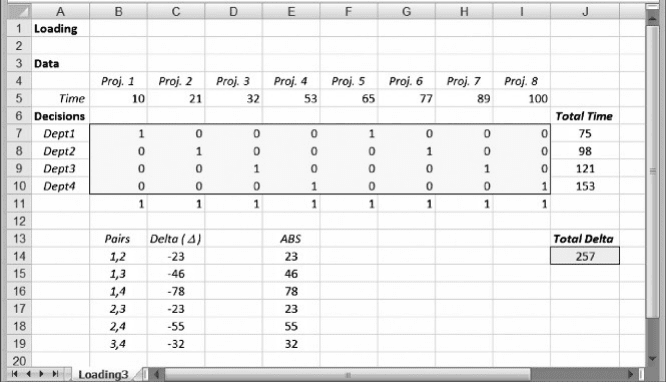
A spreadsheet model for assigning the projects to the four departments is shown
in Figure 8.18. The difference between this worksheet and the one shown in
Figure 8.16 lies only in the objective function. The decision variables in rows 7 –10
play the same role as in the previous model. Below the decision variables, in
column B, we list the six department pairs, and in column C we record for each
pair the difference in their workloads. The absolute values of these differences
appear in column E, and the total of these absolute differences serves as the objective
function in cell J14 with the formula
¼ SUM(E14:E19).
We specify the problem as follows.
Objective: J14 (minimize)
Variable: B7:I10
Constraints: B11:I11 ¼ 1
B7:I10 ¼ binary
Figure 8.18. Spreadsheet for Example 8.7 with absolute value objective.
8.5. Linearizations 325