Baker K.R. Optimization Modeling with Spreadsheets
Подождите немного. Документ загружается.


year based on a continuation of last year’s policy. This includes a new high of $38,000 in mar-
keting expense, but Manisha’s boss intimated that this might be excessive.
Late last week, Manisha read an internal marketing study that had been completed at Delhi
Foods. The study concluded that it is possible to represent the influence of marketing expenses
on demand by means of the equation
D ¼ aM
b
where D and M represent demand and marketing expenses, respectively, and where a is called
the scale factor and b the elasticity of marketing expenses. Manisha knows from courses she has
taken that this model belongs to a family of demand equations commonly used in market analy-
sis. To determine values for the parameters a and b that apply to this product, she will have to
match this model to the observations as closely as possible.
Manisha ponders the information in the table. Costs for the coming year appear to be
known; therefore, variable costs have already been estimated. Overhead and fixed production
costs do not appear to be variable costs, so they don’t enter into a calculation of gross
margin. Instead, the gross margin is based on revenue, materials costs, and other variable
costs. Using the projected figures for the coming year, Manisha expects that she will be able
to compute the gross margin per unit. From there, Manisha believes she can represent profit
for the line of dinners by using the gross margin per unit along with an estimate of demand
to predict this year’s gross margin. Then she can subtract marketing expenses and fixed costs
to arrive at a profit figure. She sees that marketing expenses show up in her profit calculation,
but they also affect her demand estimate. If she can sort out all the relationships in a spreadsheet
model, Manisha believes that she can find the optimal level to spend on marketing.
EXHIBIT 8.1 Summary of Product Costs and Revenues
Year 123456 7
Demand (cartons) 3200 3400 3500 3600 3800 4400 4700
Revenue $(000) 62,000 63,000 66,000 75,000 86,000 98,000 105,000
Production
Materials 27,000 29,000 30,000 35,000 39,000 33,000 35,000
Other variable 1700 2200 2800 3500 2400 10,800 11,600
Fixed 4500 4700 4900 5000 5300 5600 5900
Marketing
Advertising 10,300 11,700 15,000 16,200 17,800 22,000 24,000
Promotion 9000 6000 4000 11,000 12,000 13,000 14,000
Overhead 6000 6000 5000 5000 5000 5000 6000
Operating margin 3500 3400 4300 (700) 4500 8600 8500
336 Chapter 8 Nonlinear Programming

Chapter 9
Heuristic Solutions with the
Evolutionary Solver
In previous chapters, we have encountered three powerful optimization procedures—
the linear solver, the branch-and-bound procedure, and the nonlinear solver. For linear
models, we use the linear solver. This algorithm is reliable: It always finds a global
optimum when the model does not contain an unbounded objective function or con-
flicting constraints. For linear programming models with integer constraints, we also
rely on the linear solver. The integer constraints are added in the problem formulation,
informing the linear solver to use its branch-and-bound procedure in the search for an
optimal solution. The branch-and-bound procedure relies on solving a series of linear
programs, so if Solver does not run out of time, this is a reliable procedure, too.
However, when the model does not satisfy the conditions of linearity, the linear
solver is of no use.
For nonlinear programming problems, we use the nonlinear solver. This algor-
ithm is not as reliable as the linear solver because it may stop its hill climbing at a
local optimum and it is unable to determine whether it has found a global optimum
or stopped short of one. We can at least improve our chances of finding a global opti-
mum by re-running the nonlinear solver from a variety of different starting points, a
process we can automate with the MultiStart option. However, when the problem is
not composed of smooth functions, the nonlinear solver often fails to help.
The fourth solution procedure in RSP is the evolutionary solver, which is the sub-
ject of this chapter. This procedure is particularly useful for tackling optimization
models containing nonsmooth functions. As suggested in Chapter 8, a nonsmooth
function is one that exhibits gaps or kinks. The presence of a nonsmooth function
undermines the performance of the linear and nonlinear solvers. However, the avail-
ability of a solution procedure suitable for nonsmooth functions allows us to build
models with more flexibility than under the restrictions of the linear and nonlinear
solvers. In particular, we can take advantage of several Excel functions in the model.
We can include the IF function, which allows us to represent some simple logical
choices. We can include several other familiar mathematical functions, such as
ABS, MIN, MAX, CEILING, FLOOR, ROUND, and INT. (Although it is sometimes
Optimization Modeling with Spreadsheets, Second Edition. Kenneth R. Baker
# 2011 John Wiley & Sons, Inc. Published 2011 by John Wiley & Sons, Inc.
337
possible to avoid using these functions directly, doing so may require the use of binary
variables or auxiliary variables in cumbersome or unusual ways.) We can also include
spreadsheet-oriented functions such as CHOOSE, COUNTIF, INDEX, and
LOOKUP, which may provide convenience in spreadsheet calculations even though
they are seldom used in other circumstances. Thus, another way of interpreting non-
smooth is any computation that uses one of these dozen functions or one of the
other specialized functions in Excel.
The modeling flexibility comes at a price. Because the evolutionary solver makes
virtually no assumptions about the nature of the objective function, it has a limited
ability to identify an optimal solution. Essentially, it conducts a search, compares the
solutions encountered as it proceeds with the search, and stops when it senses that it is
making very little progress at finding improvements. The solution it generates may not
even be a local optimum, such as the solution the hill-climbing procedure delivers, yet
in many kinds of problems, the evolutionary solver delivers a good solution, if not an
optimal one. This type of procedure is called a heuristic procedure, meaning that it is a
systematic procedure for seeking good solutions, but it cannot guarantee optimality.
9.1. FEATURES OF THE EVOLUTIONARY SOLVER
A few features of the evolutionary solver are helpful to know. First, it is important
to realize that the procedure contains some randomized steps. As a consequence, we
may get different solutions when we run the evolutionary solver twice on exactly
the same model.
The evolutionary solver works with a population of solutions. At intermediate
stages of the solution procedure, it keeps track of several solutions rather than main-
taining just the one, best solution found so far. This population of solutions develops,
or evolves, in steps that mimic naturally occurring evolutionary processes. From the
population of solutions that it builds and maintains, the procedure can generate new
solutions, following the principle that an offspring solution should combine traits
from each of two parent solutions. In addition, there are occasional mutations,
which are offspring solutions with some random characteristics that do not come
from their parents. Over the course of the procedure, the population is governed by
a fitness criterion (based on the objective function) that removes the poorer solutions
and keeps the better ones. This process of selection drives the population toward better
levels of fitness (better values of the objective function). If there is evidence that the
population is no longer improving, or if one of the user-designated stopping conditions
is met, then the procedure stops. When it stops, Solver displays the best member of the
final population as the solution.
The inner workings of the evolutionary solver do not concern us at this stage.
However, in the next section, we provide an example that will help explain concep-
tually how the procedure works. The main point is that the evolutionary solver is
not handicapped by the presence of nonsmooth functions, as would be the case for
the linear and nonlinear solvers. It is also helpful to set some user-controlled options
when running the evolutionary solver. However, in the end, the evolutionary solver
cannot guarantee that it has found a global optimum, so some judgment is
338
Chapter 9 Heuristic Solutions with the Evolutionary Solver

required—even more than with the nonlinear solver—when applying it to a particular
optimization problem.
In this chapter, we examine a series of examples that contain nonsmooth func-
tions, to illustrate how the evolutionary solver works. In some cases, we revisit pro-
blems that we tackled with other solution procedures in earlier chapters, mainly to
provide a contrast in optimization approaches. The variety of examples should provide
a working knowledge of the evolutionary solver, but, more than the other solvers we
have covered, this one requires practice and experience in order to use it effectively.
9.2. AN ILLUSTRATIVE EXAMPLE: NONLINEAR
REGRESSION
As our first example, we look at a curve-fitting problem in which the relationship
between two variables is nonlinear and in which the criterion is the sum of absolute
deviations. As discussed in Chapter 8, the most appropriate tool for curve-fitting pro-
blems is the nonlinear solver when the criterion is the sum of squared deviations. But
when the criterion is the sum of absolute deviations, several local optima may exist,
and the nonlinear solver may not find the best fit. The evolutionary solver is often
well suited to such problems.
Our purpose here is to describe, in an approximate way, how the evolutionary
solver works. This is not meant to be a precise description of the algorithm, but rather
a suggestive description of the evolutionary approach and the elements it contains. For
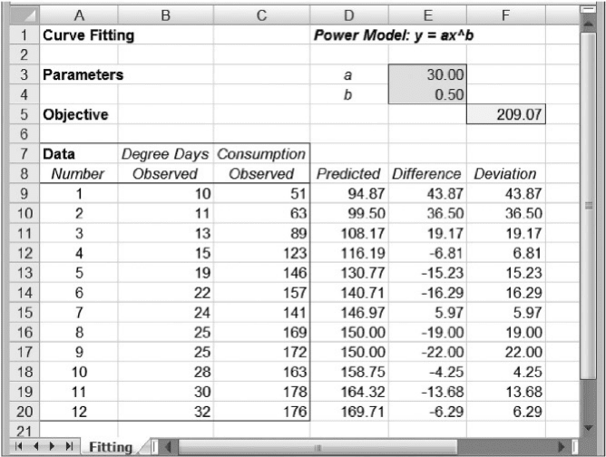
a specific example, we revisit the data from Fitzpatrick Fuel Supply (Example 8.3),
where we wanted to predict gas consumption on the basis of degree days.
Data from Example 8.3
A sample of 12 observations was made at customers’ houses on different days and the following
observations of degree days and gas consumption were recorded.
Degree Gas
Day days consumption
110 51
211 63
313 89
4 15 123
5 19 146
6 22 157
7 24 141
8 25 169
9 25 172
10 28 163
11 30 178
12 32 176
9.2. An Illustrative Example: Nonlinear Regression
339
As a first cut at the estimation problem, Fitzpatrick’s operations manager would like to fit a
linear model to the observed data.
Fitzpatrick’s operations manager believes that the power curve, y ¼ ax
b
is a good
model. As a criterion, suppose that we want to minimize the sum of absolute devi-
ations (instead of squared deviations) between model and observations. This is a
less common criterion than the sum-of-squares measure that was used in Chapter 8,
but it is just as plausible for optimization purposes. Whereas the sum-of-squares
measure penalizes large deviations more severely than small ones, that is not the
case for the absolute-deviation measure.
Figure 9.1 displays a worksheet for this problem. The given data, consisting of 12
observations, can be found in the first three columns. The parameters a and b, which
serve as the decision variables, are located in cells E3 and E4. Specifying these two
parameters allows us to generate the values found in the column labeled Predicted
in column D, and the differences between model and observation are calculated in
column E. The absolute value of this difference appears in the next column, under
the heading Deviation. The sum of these absolute deviations, which is the objective
function to be minimized, appears in cell F5.
Knowing a little about the range of observations, we can make an educated guess
that the best value of a lies between 0 and 50, while the best value of b lies between
0 and 1. These are coarse limits, but they are sufficient to get us started. We generate an
Figure 9.1. Spreadsheet model for Example 8.3.
340 Chapter 9 Heuristic Solutions with the Evolutionary Solver

initial set of pairs (a, b) by sampling randomly from these two ranges. Let’s suppose
this process generates the values shown in Table 9.1. In each case, the fitness number is
the objective function that corresponds to the values of a and b, and this value can be
calculated directly by using the worksheet. Here, we have constructed a population of
size 6. The best fitness is 440, and the average fitness is about 1706.
Next, we create new members of the population by the crossover method. In par-
ticular, we take the first two solutions and swap their a values. That way, the a value of
the first solution is paired with the b value of the second solution, and vice versa. In
other words, the two new solutions are (30.8, 0.55) and (19.7, 0.19). We can think of
these two solutions as being “offspring” of the original two solutions, with values of a
and b (interpreted as genes) that are inherited from their “parents.”
Suppose that the next new member of the population is created by the mutation
method. For the third solution, we keep the second gene (b) and randomly generate
the first gene (a), obtaining (20.0, 0.82)
Next, we’ll perform the crossover step on solutions 4 and 5, and then generate
another mutation from the sixth solution by keeping the first gene and randomly
generating the second. The six new members are shown in Table 9.2.
We can think of this list as newcomers to the population in one generation or
cycle. We’ll combine these members with the existing members and apply the fitness
criterion. This means that we’ll select a second generation of size 6, keeping just the
six best fitness values. The list becomes Table 9.3.
The best fitness in the new population has dropped from 440 to 322, and the aver-
age fitness has dropped from 1706 to 684.
Table 9.1. Initial population
abFitness
30.8 0.19 975
19.7 0.55 440
47.2 0.82 5230
30.0 0.59 519
43.8 0.66 2257
7.6 0.72 817
Table 9.2. First generation of offspring
abFitness
30.8 0.55 322
19.7 0.19 1210
20.0 0.82 1278
30.0 0.66 1033
43.8 0.59 1506
7.6 0.45 1273
9.2. An Illustrative Example: Nonlinear Regression
341

To create the third generation, we follow a similar procedure. We use the first two
solutions as parents to generate two offspring by the crossover operation. We use the
third solution to generate a mutation by randomly replacing the a value. Then we
repeat the process, applying the crossover operation to the fourth and fifth solutions,
and generating another mutation by randomly replacing the b value in the sixth sol-
ution. The six new members of the populations are shown in Table 9.4.
Combining this list with the previous one, we use the fitness criterion to remove
the least-fit members of the population, thus selecting the six best solutions as the third
generation (Table 9.5).
Now, the best solution in the population has improved to 217, and the average has
dropped to about 417. Another generation leaves the best solution unchanged but the
average drops to about 352.
Table 9.3. Population updated for fitness
abFitness
30.8 0.19 975
30.0 0.59 519
30.8 0.55 322
19.7 0.55 440
7.6 0.72 817
30.0 0.66 1033
Table 9.4. Second generation of offspring
abFitness
30.8 0.59 576
30.0 0.19 992
17.8 0.55 533
19.7 0.72 474
7.6 0.55 1147
30.0 0.54 217
Table 9.5. Second updated population
abFitness
30.0 0.54 217
30.8 0.55 322
19.7 0.55 440
19.7 0.72 474
30.0 0.59 519
17.8 0.55 533
342 Chapter 9 Heuristic Solutions with the Evolutionary Solver
As these first few iterations suggest, the crossover and mutation procedures, along
with the fitness criterion, tend to generate populations with improving fitness values.
Clearly, a generation of solutions always has a best value and an average value that are
no worse than those of the previous generation. As we continue the process, which
Solver can do at great speed, we tend to find additional improvements.
The evolutionary solver does not follow the precise details of the generation-
building process we have outlined here, although it does rely on the crossover and
mutation procedures. The details of the actual implementation are not important in
order to understand how to implement the evolutionary solver, but here are some
relevant observations.
†
For the purposes of implementing the crossover operation, the specific form of
a gene depends on the model and is determined within the evolutionary solver.
†
The frequency with which mutations appear is an option set by the user. The
genetic form of a mutation, however, is determined within the evolutionary
solver.
†
The procedure contains some randomness, so two successive runs from the
same starting point can produce different solutions.
†
There can be no guarantees of optimality; the procedure may stop short of find-
ing an optimum.
To understand how the procedure stops, let’s look at the various options available
when we implement the evolutionary solver on a particular model.
In the task pane, we select the Standard Evolutionary Engine from the drop-
down menu on the Engine tab. Some elements that appear in the task pane are tailored
to the evolutionary solver, whereas others are common to the linear solver and the
nonlinear solver as well. For example, the Max Time parameter limits the amount
of time Solver uses trying to find a good solution before stopping. Normally, we
use this option as a kind of last resort. It should be set long enough that other options
have an opportunity to take effect, and it should reflect the amount of time we are will-
ing to allow the procedure to run without intervening. For large and complicated pro-
blems, this could mean a long wait, but we often choose a short time limit so that we
can get feedback quickly. When debugging a model, or just trying to get a feel for per-
formance on a given model, we might set this option to 20 or 30 seconds.
The user can also set the Population Size parameter. The purpose here is to make
sure that the population is sufficiently diverse. We used a population of size six in our
curve-fitting example, but that would be small for the automated implementation used
by Solver. In the course of solving a particular problem, we might start with a value as
small as 25 and later try a larger value for greater diversity. The evolutionary solver
will stop (with a convergence message) when 99 percent or more of the population
has fitness values whose relative differences are less than the Convergence parameter
shown in the task pane. A population size no more than 200 is required, but 50 might
often be adequate for even very difficult problems.
The Mutation Rate parameter affects the level of randomness in generating new
members of the population. A low rate would create few mutations, whereas a high rate
9.2. An Illustrative Example: Nonlinear Regression 343

offers greater diversity. The default value is 7.5 percent. We might raise this value if
we find evidence that the evolutionary solver stalls due to lack of diversity. As in our
example, the population may gravitate toward a set of similar solutions. When that
type of population convergence begins to take place, we may be located near a
global optimum, and our chances of locating that optimum become high. Raising
the mutation rate in such a case is unlikely to produce much improvement. On the
other hand, when convergence occurs at some distance away from a global optimum,
the process is analogous to finding a local optimum with the nonlinear solver. In that
case, we’d want to increase the diversity in the population, and it would be desirable to
raise the mutation rate. Normally, we do not know whether we are close to a global
optimum, but the effect of raising the mutation rate may provide a clue.
Another option is the Require Bounds option, asking whether to require upper and
lower bounds on the decision variables. This option should set to True, meaning that
the model must contain at least simple bounds entered as constraints. One of the
bounds may be dictated by a nonnegativity requirement, which is most conveniently
implemented by setting the Assume Non-Negative option to True. The evolutionary
solver tends to work more efficiently when the decision variables are bounded.
Finally, in the Limit section of the task pane, we encounter additional parameters.
The first two options in this section are the Max Subproblems parameter and the Max
Feasible Solutions parameter, both of which can limit the amount of effort Solver
devotes to a problem before stopping. However, these parameters can be left blank
as long as the Max Time parameter is set.
The next pair of options in the Limits section work together. They specify that the
search should stop if an improvement of at least the Tolerance has not been found in
the last Max Time without Improvement. It’s usually convenient to keep the Tolerance
at 0 percent but to vary the time without improvement according to previous outcomes.
The list in Box 9.1 describes particular settings that would be appropriate in the
initial stages of using the evolutionary solver. Some of the values are Solver default
values, while others are entered by the user, in some cases overriding the default
values. In addition, the Nonsmooth Mode l Transformation option, which appears
on the Platform tab of the task pane, should be set to Never. (Otherwise, Solver
may add some variables and constraints to the model that undermine the effectiveness
of the evolutionary solver.)
Returning to our example of nonlinear regression, suppose we set the initial
values of the decision variables to a ¼ 30.0 and b ¼ 0.50 and set the Assume
BOX 9.1
Initial Values for Parameters in the Evolutionary Solver
Max time: 30 sec Population Size: 25
Convergence: 0.0001 Mutation rate: 7.5%
Tolerance: 0 Max time w/o improvement: 15 sec
344 Chapter 9 Heuristic Solutions with the Evolutionary Solver

Non-negative option to True (so that we have lower bounds on both decision vari-
ables). We specify the problem as follows.
Objective: F5 (minimize)
Variables: E3:E4
Constraints: E3 50
E4 1
For the sake of comparison, we might initially run the nonlinear solver. It produces a
solution with a total absolute deviation of 173.41. We turn now to the evolutionary
solver.
Due to randomness, we may not find that any two runs of the evolutionary solver
match exactly, but in this case, the results are similar. Suppose we initialize the model
with the decision variables shown in cells E3 and E4 of Figure 9.1. Two runs stop with
an objective function value of 160.10 and the following message in the Output
window.
Solver cannot improve the current solution.
All constraints are satisfied.
This “improvement” message means that no improvements were encountered in the
last 15 seconds of searching. This stopping condition occurred within the 30-
second Max Time limit.
The third run reaches the 30-second Max Time limit and produces a window with
the message: The maximum time limit was reached; continue anyway? At this stage,
the user can choose whether to continue or stop. When we press the Stop button, the
run terminates. The solution happens to again be 160.10 and the following message
appears in the Output window.
Stop chosen when the maximum time limit was reached.
From these results, it is difficult to determine how close we might be to an optimal
solution. Because the time-limit parameters limited the search, we might re-run the
evolutionary solver with a Max Time parameter of 60 seconds and a Max Time with-
out Improvement parameter of 30 seconds. If we find no improvements, we might try a
larger population size or a larger mutation rate, but in this case no improvements occur.
Although we have no guarantee, the evidence suggests that further searching will not
turn up an objective function value lower than 160.10. Figure 9.2 shows the best
solution found during the last run of the evolutionary solver.
Our example of nonlinear regression served two purposes. First, it allowed us to
use a manual method to describe the main workings of the evolutionary solver—cross-
overs, mutations, and selection by a fitness criterion. Second, it illustrated a straight-
forward optimization problem in which the nonlinear solver may not work as well as
the evolutionary solver. This is partly due to the existence of many local optima in the
example, but it’s also true that evolutionary methods have proven particularly effective
on complex regression problems. In the examples that follow, we focus more on the
model than on the refinements needed in the options to produce a good solution.
9.2. An Illustrative Example: Nonlinear Regression 345