Baker K.R. Optimization Modeling with Spreadsheets

Подождите немного. Документ загружается.

9.3. THE MACHINE-SEQUENCING PROBLEM

REVISITED

In the machine-sequencing problem, a set of jobs is waiting to be processed. The

machine can work on only one job at a time, so the jobs must be processed in

a sequence. The problem is to ﬁnd the best sequence for a given objective

function. In Chapter 7, we saw how to build an integer programming model for this

problem. That model requires a number of disjunctive constraints to accommodate

the conditions of feasibility. An alternative approach is available if we use the evol-

utionary solver.

We revisit the Miles Manufacturing Company (Example 7.4), in which we have

six jobs waiting to be scheduled. Each job will be either on time or late, depending on

the sequence chosen. If a job is late, the amount of time by which it misses its due date

is called its tardiness. Tardiness is zero when a job completes prior to its due date. The

objective is to minimize the total tardiness in the schedule.

Data from Example 7.4

This morning’s workload consists of six jobs, as described in the following table.

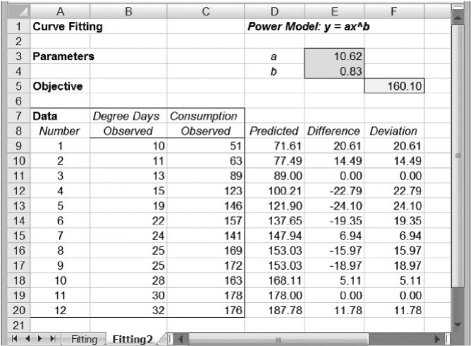
Figure 9.2. Best solution found for Example 8.3.

346 Chapter 9 Heuristic Solutions with the Evolutionary Solver

Job number 123456

Processing time (hours) 5 7 9 11 13 15

Due date (hours from now) 28 35 24 32 30 40

The problem is to sequence the six jobs so that work can begin.

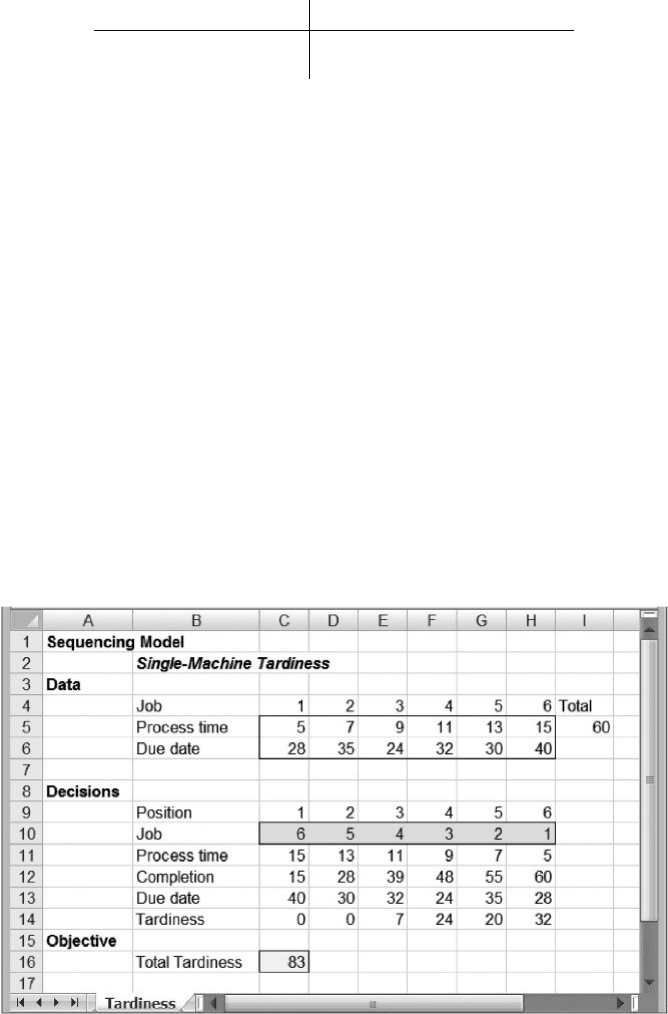
Figure 9.3 displays a model for this problem. The ﬁrst module contains the tabu-

lated data describing the speciﬁc problem to be solved. The next module contains a

row of decision variables corresponding to the job sequence. Each position in

sequence is assigned a job number (from 1 to 6). Since the sequence does not necess-

arily match the numbered sequence in which the data appear, we use the INDEX func-

tion to access the processing times and due dates that match the job in each sequence

position. For example, the formula in cell C11, for the processing time of the ﬁrst job,

¼ INDEX($C$4:$H$6,2,C$10). The INDEX function references the element

in the second row of the data in the column corresponding to the number in C10. A

similar function in cell C13 references the third row of the data, with the formula

¼ INDEX($C$4:$H$6,3,C$10).

The processing times and due dates thus appear in rows 11 and 13. From the pro-

cessing times, we can compute the completion times directly, as shown in row 12. In

row 14, we compute tardiness values, working from the completion time and due date

in the two rows directly above and using the formula

¼ MAX(0,C12-C13) in cell

C14, and then copying the formula to the right. We sum the tardiness values in cell

C16; this total represents the value of the objective function.

Figure 9.3. Spreadsheet for Example 7.4.

9.3. The Machine-Sequencing Problem Revisited 347

In the cells corresponding to decision variables, we want to choose integers

between 1 and 6. Therefore, our ﬁrst instinct might be to add constraints that restrict

the decision variables to integers no less than 1 and no greater than 6. However,

those constraints permit the choice of some jobs more than once. We would have to

add a module that tests for duplication and penalizes solutions that choose any job

multiple times. Wouldn’t it be nice if we could avoid the intricacies of this inefﬁcient

ﬁltering device and generate only solutions for which the integers in the decision cells

contain no duplicates?

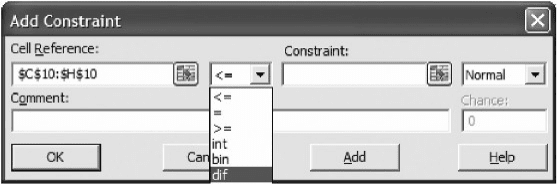
The capability we seek is usually called an alldifferent constraint: It ensures that

the values of the decision variables form a set of integers with no duplicates. To

implement the alldifferent constraint, we enter the cell range as the left-hand side

and then use the drop-down menu of constraint types to select dif, as shown in

Figure 9.4. The alldifferent constraint ﬁlls the designated range of cells with the inte-

gers from 1 to n in some order, where n is the number of cells in the range.

A comparison with the integer programming model of Figure 7.14 shows that the

evolutionary solver model is more compact and easier to understand. Its layout on the

worksheet resembles the calculations we might make if we were verifying the value of

total tardiness with pencil-and-paper calculations. However, because the objective

function relies on the INDEX function and on the MAX function, it is a nonsmooth

model and cannot be solved using the linear solver.

We specify the problem as follows.

Objective: C16 (minimize)

Variables: C10:H10

Constraints: C10:H10 ¼ alldifferent

We run the evolutionary solver, starting arbitrarily with the solution 6-5-4-3-2-1 and

using the default options. The procedure may examine several thousand solutions, or it

may terminate due to the Convergence criterion. When we run the model again, start-

ing with the sequence generated by the previous run, we may get a better solution. This

cycle can be repeated if improvements are found. If not, we can try modifying the

initial sequence and re-running Solver. After a few trials of this sort, Solver is likely

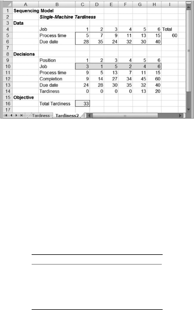
to produce the solution shown in Figure 9.5, with a value of 33. We recognize this

as the optimal value, from our work in Chapter 7. There is no guarantee, however,

that another run of the very same model will terminate with this solution.

Figure 9.4. Specifying the alldifferent constraint.

348 Chapter 9 Heuristic Solutions with the Evolutionary Solver

9.4. THE TRAVELING SALESPERSON PROBLEM

REVISITED

We encountered the traveling salesperson problem in Chapter 7, and we saw how to ﬁnd

optimal solutions by starting with an assignment model and appending subtour

elimination constraints as needed. This approach required the solution of a series of

integer programs with an unpredictable number of constraints. For large problems,

the manual task of keeping track of the appended constraints could be daunting even

if the resulting integer programming problems could be solved in a reasonable

amount of time. As an alternative, we look at a solution approach that relies on the

evolutionary solver, revisiting the Douglas Electric Cart Company (Example 7.5).

Data from Example 7.5

In today’s schedule, there are six colors (C1 –C6) with cleaning times as shown in the table

below.

C1 C2 C3 C4 C5 C6

C1 –16632120 6

C257 –40466942

C3 23 11 – 55 53 47

C4 71 53 58 – 47 5

C5 27 79 53 35 – 30

C6 57 47 51 17 24 –

Figure 9.5. Final solution for Example 7.4.

9.4. The Traveling Salesperson Problem Revisited 349

The entry in row i and column j of the table gives the cleaning time required between product

batches of color Ci and color Cj. Each production run consists of a cycle through the full set of

colors, and the operations manager wishes to sequence the colors so that the total cleaning time

in a cycle is minimized.

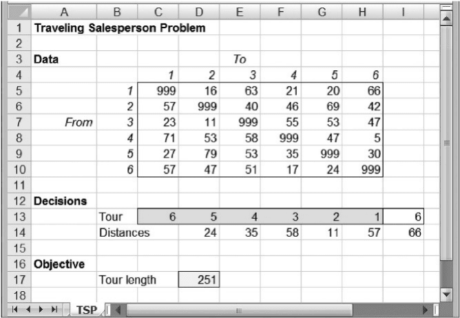
Using the evolutionary solver, our formulation can be much more compact and

readable than the integer programming model. Figure 9.6 displays a spreadsheet

model for Example 7.5. The ﬁrst module contains the distance array, which serves

as the given data for the problem. Then, in the second module, the decision variables

are listed in row 13, comprising the sequence of cities in the tour. For an n-city pro-

blem, this simply means a single row listing the integers from 1 to n, in some order.

By deﬁnition, a tour must return to its starting point, so we repeat the starting city

in cell I13. (This cell is not a decision variable; it is simply a reference to cell C13.)

Directly below the cells of the tour, we capture the distances between pairs of

cities on the tour, as shown in Figure 9.6. Again, we can use the INDEX function

for this purpose. For example, the distance corresponding to the pair in cells

C13 and D13 is isolated in cell D14 with the formula

¼ INDEX($C$5:

$H$10,C13,D13)

, which is copied to the right. In the third module, consisting of

cell D17, we compute the sum of the pairwise distances calculated in row 14. This

sum represents the total tour length.

The inputs and the outputs of this calculation are more natural than in the case

of an integer programming formulation. In addition, the spreadsheet is easier to

Figure 9.6. Spreadsheet model for Example 7.5.

350 Chapter 9 Heuristic Solutions with the Evolutionary Solver

understand on its face. However, because we use the INDEX function as a component

in the objective function, this is a nonsmooth model, and it is not appropriate for either

the linear solver or the nonlinear solver.

We specify the problem as follows.

Objective: D17 (minimize)

Variables: C13:H13

Constraints: C13:H13 ¼ alldifferent

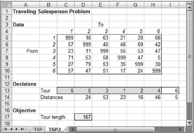
Even with the default settings, we are likely to obtain a solution of 167, as shown in

Figure 9.7. (In Chapter 7, we found that this value was optimal.) The evolutionary

solver rather quickly ﬁnds the tour 6-5-3-1-2-4, which matches the optimal tour found

in Chapter 7. (Starting the tour at city 1 corresponds to the solution 1-2-4-6-5-3-1.)

Is the evolutionary solver always capable of ﬁnding an optimum with such limited

effort? Unfortunately, it’s not. It is difﬁcult to generalize about the effectiveness of the

evolutionary solver on sequencing problems, but some experience suggests that pro-

blems of ﬁnding the best sequence can be solved to optimality with modest effort if

the sequence length is 10 or sometimes 15. In the traveling salesperson problem, as

in the machine sequencing problem, the model is simpler and the solution is obtained

more quickly using the evolutionary solver than with an integer programming

approach. However, the evolutionary solver cannot guarantee optimality. Next, we

turn to problems that we have not previously solved, so that we will not know the opti-

mum when we set out to ﬁnd a solution.

Figure 9.7. Final solution for Example 7.5.

9.4. The Traveling Salesperson Problem Revisited 351

9.5. TWO-DIMENSIONAL LOCATION

In many location decisions, costs are mainly determined by geographic distances, and

it is possible to gain some insight into location possibilities by building models based

on the geometry of physical location. Consider the location problem facing Drezner

Chemical Company.

EXAMPLE 9.1

Drezner Chemical Company

Drezner Chemical Company delivers its products to 10 ﬁrms in the wholesale chemicals

business and will continue to do so when its new plant comes on line and replaces current pro-

duction. The actual customers who use Drezner’s products can be classiﬁed into clusters, with

each cluster serviced by a single wholesaler. From Drezner’s point of view, however, each clus-

ter represents one demand source because each wholesaler handles the logistics for all of the

customers in its cluster. The transportation cost for the new plant will be related to the distances

between the plant and each of the clusters. Since the wholesalers are responsible for the logistics

within each cluster, Drezner delivers to the nearest member of the cluster. Truck capacity will

not be a factor in the foreseeable future.

The customer base is spread out over the state, which to good approximation can be viewed

as a square, 100 miles on each side. Each customer within each cluster has a location in that

square, denoted by the (x, y) pair on a graph that has a lower left-hand point at the origin and

an upper right hand point at (100,100). There are 10 customers in each cluster.

Drezner makes one round-trip delivery to each cluster every week. The distance for a round

trip is twice the distance from the plant to the nearest point in the cluster. The Euclidean distance

metric applies: if (x

, y

) denotes the location of cluster k, then the distance to cluster k from the

plant at (x, y) is given by

(x, y) ¼ [(x  x

)

þ ( y  y

)

]

1=2

Based on this geometric model, Drezner wishes to ﬁnd the optimal location for its plant. B

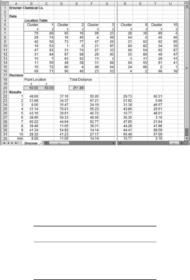
A model for the problem is shown in Figure 9.8, with some columns omitted. The

ﬁrst module contains the customer location data—100 pairs of (x, y) values describing

each customer’s location, organized into 10 sets for each of 10 clusters. The second

module contains the decision about the plant’s location, represented by x- and y-

coordinates in cells B20:C20. This module also contains the objective function. The

Results module contains distances from the plant to each of the 100 customers,

again organized in 10 sets of 10. At the bottom of the Results module, we calculate

the minimum distance in the cluster, and the objective function (cell E20) sums the

lengths of the 10 distances and multiplies by two to account for round trips.

We specify the model as follows.

Objective: E20 (minimize)

Variables: B20:C20

Constraints: B20:C20  100

B20:C20  0

352

Chapter 9 Heuristic Solutions with the Evolutionary Solver

The last of these constraints can be omitted if we check the option for Assume Non-

Negative instead. But in any case, this model is ready for the evolutionary solver.

It is instructive to attack this problem with the nonlinear solver. Although the

reliance on the square-root formula for distances might suggest that the nonlinear

solver should work effectively, it turns out that the solution is sensitive to the starting

point, and several local minima exist. The table below lists ﬁve cases, showing the

starting point, the solution produced by the nonlinear solver, and the corresponding

value of the objective function.

Starting Local Solution

solution optimum value

(40, 60) (23.00, 53.00) 266.12

(45, 55) (48.32, 48.75) 250.60

(50, 50) (49.09, 49.92) 251.32

(55, 45) (48.32, 48.75) 250.60

(60, 40) (48.32, 48.75) 250.60

We might be inclined to conclude that the optimal location is in the vicinity of

(50, 50), with an objective function value close to 250. However, we discover a

different story when we use the evolutionary solver.

Figure 9.8. Spreadsheet model for Example 9.1.

9.5. Two-Dimensional Location 353

When we switch to the evolutionary solver, we are very likely to ﬁnd improve-

ments. Recall that there is some built-in randomness and the evolutionary solver

does not necessarily stop with the same solution each time. In addition, the developers

of the evolutionary solver offer the following advice for producing solutions.

†

Restart the evolutionary solver, using the solution it produced on the ﬁrst run, to

see if an improvement can be found.

†

Restart the evolutionary solver with changes in the Convergence value (tighter)

or the Tolerance value (tighter, if it’s not already zero).

†

Restart with a larger Population Size parameter and/or a larger Mutation Rate

parameter. These changes will result in longer runs, and they tend to examine a

larger number of candidate solutions.

†

Switch to the nonlinear solver and see whether it can produce an improvement.

Finally, some insight may come from examining Solver’s Population Report. Stability

in the Best Values and relatively small Standard Deviations are signs to look for. Those

signs suggest little room for improvement.

Using just the ﬁrst of the listed suggestions, and restarting Solver a few times, we

are likely to encounter a solution that is signiﬁcantly better than those found with the

nonlinear solver. For example, the evolutionary solver may ﬁnd the objective function

value of 217.61 at a plant location of (87.33, 53.43). By using the evolutionary solver,

Drezner can ﬁnd a location that improves on the solution generated by the nonlinear

solver. If the distance metric is a good proxy for annual distribution expenses,

Drezner will be able to reduce its expenses more than 13 percent by using the evol-

utionary solver, as compared to the decisions it would have reached using the non-

linear solver.

9.6. LINE BALANCING

The line-balancing problem arises in the design of a new production process for

assembled products. Examples might include home appliances (refrigerators), elec-

tronics (televisions), light vehicles (lawn mowers), and automobiles. At the end of

the product design phase, the product and its components are well known, and so

are the speciﬁc tasks that must be carried out to make the product. The next step is

to design the production line on which the product will be assembled.

The ﬁrst type of information is the time required for each task. Required times

might be based on previous experience with the same task in other lines or estimated

by experts in work measurement techniques. The second type of information is pre-

cedence information. In other words, we need to know which tasks must be completed

before some other task can begin. We say, “task j precedes task k” to mean that k

cannot begin until j is completed. Precedence information can be expressed in a list

or in a diagram.

The production line typically has a target output rate—so many units per hour.

The cycle time is the inverse of the output rate. For example, if we specify a target

of ﬁve units per hour, the cycle time is 1/5 of an hour, or 12 minutes.

354

Chapter 9 Heuristic Solutions with the Evolutionary Solver

The physical production line consists of several work stations, typically numbered

according to their position along the line. At each station, a single operator carries out a

set of tasks. The problem is to assign the various tasks to stations. The criterion is to

use as few stations as possible, since the number of stations dictates the number of

operators, and therefore the labor cost per unit. There are essentially two types of con-

straints. First, the amount of work assigned to any individual station may not exceed

the cycle time; otherwise, the target production rate cannot be met. Second, no task can

appear earlier in the line (i.e., at a lower-numbered station) than any of its predecessor

tasks. An example arises at Munoz Manufacturing Company, in the assembly of

microwave ovens.

EXAMPLE 9.2

Munoz Manufacturing Company

Along with the design of a new countertop oven, the manufacturing engineers at Munoz

Manufacturing Company have determined the 12 distinct tasks that comprise the assembly

process. They have summarized this information in a table showing the time for each task

and its logical predecessors—that is, the tasks that must be done earlier in the process.

Predicted volume targets have been translated into a desired cycle time of 15 minutes. The

following table shows the relevant information.

Task Time Predecessors

112 –

26 1

36 2

42 2

52 2

612 2

77 34

85 7

91 5

10 4 6 9

11 6 8 10

12 7 11

To complete the design of the production process, the individual tasks must be assigned

to stations, respecting the desired cycle time and minimizing the number of stations

required.

The precedence relations among activities in a line-balancing problem present

a signiﬁcant challenge in formulating and implementing an optimization model.

Moreover, optimization models usually require a large number of variables for a

design of realistic scale. For those reasons, line-balancing problems are often solved

by heuristic methods. Here, we describe an approach to solving the line-balancing

problem that relies on the evolutionary solver.

9.6. Line Balancing 355