Balakumar Balachandran, Magrab E.B. Vibrations
Подождите немного. Документ загружается.

120 CHAPTER 3 Single Degree-of-Freedom Systems
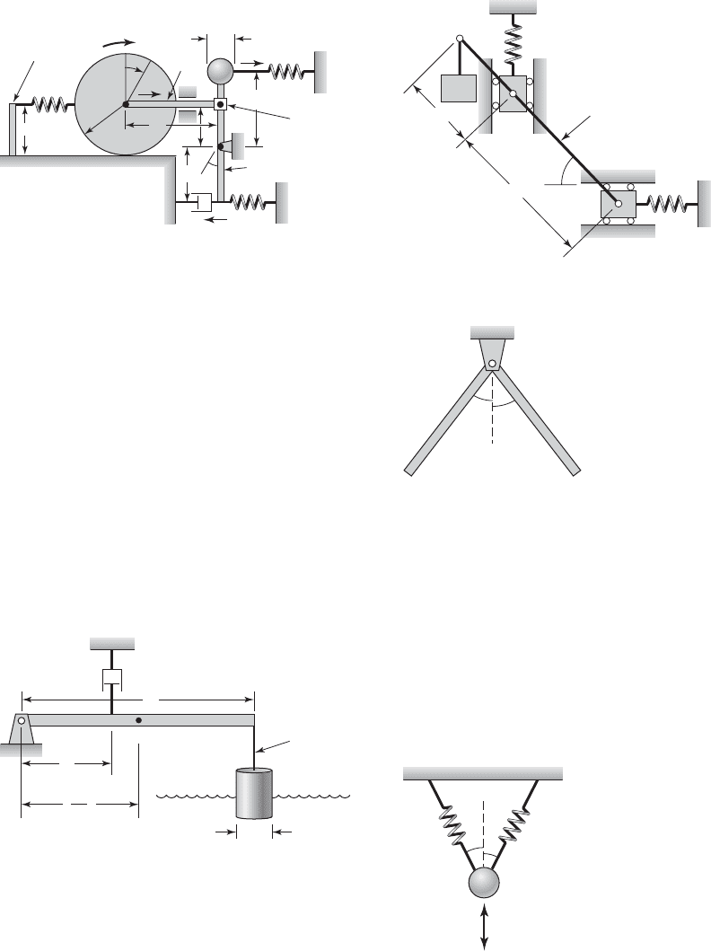
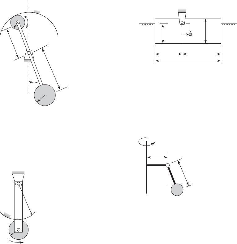
3.32
Determine the nonlinear governing equation of
motion for the kinematically constrained system
shown in Figure E3.32. Consider only vertical mo-
tions of m
1
.
each uniformly distributed. The cylinder rolls without
slipping. The rotational inertia J
c
of the cylinder is
about the point O and J
sp
is the total rotational inertia
of the rod about the point s. Assume that these rota-
tional inertias are known.
3.31 For the fluid-float system shown in Figure E3.31,
J
o
is the mass moment of inertia about point O.Assume
that the mass of the bar is m
b
. Answer the following.
a) For “small” angular oscillations, derive the govern-
ing equation of motion for the fluid float system.
b) What is the value of the damping coefficient c for
which the system is critically damped?
3.33 Determine the natural frequency of the angle
bracket shown in Figure E3.33. Each leg of the
bracket has a uniformly distributed mass m and a
length L.
3.34 Determine the natural frequency for the vertical
oscillations of the system shown in Figure E3.34. Let
L be the static equilibrium length of the spring and let
. The angle g is arbitrary. x/L 1
FIGURE E3.33
FIGURE E3.34
kk
x
m
FIGURE E3.32
k
2
k
3
m
3
m
2
Rigid, weightless rod
a
b
m
1
FIGURE E3.31
L
c
c.g.
J
o
d
O
a
Rigid, weightless
connection
m
L
2
FIGURE E3.30
r
M(t)
2a
2r
k
1
Cantilever
beam
Cylinder
Knuckle slides
on pendulum
and pivots with
respect to m
r
x
3
x
2
L
2
L
3
L
1
c
k
3
k
2
J
c
, m
c
m
a
m
r
s
J
sp
, m
p
r
O
x
c
Exercises 121
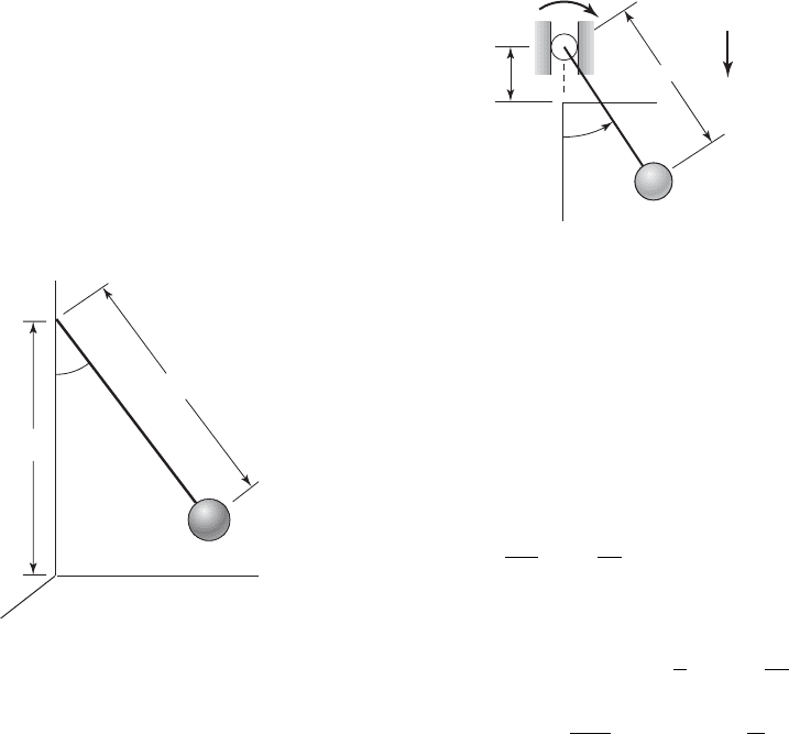
3.35
Consider the planar pendulum of mass m and con-
stant length l that is shown in Figure E3.35. This
pendulum is described by the following nonlinear
equation
where u is the angle measured from the vertical. De-
termine the static-equilibrium positions of this system
and linearize the system for “small” oscillations about
each of the system static-equilibrium positions.
ml
2
u
$
mgl sin u 0
FIGURE E3.35
Z
X
P
O
h
Q
L
Y
At the point about which the pendulum rotates, there
is a viscous damping moment .
a) Determine expressions for the kinetic energy and
the potential energy of the system.
b) Show that the governing equation of motion can be
written as
where
c) Approximate the governing equation in (b) for
“small” angular oscillations about u
o
0 using a
two-term Taylor expansion for sin u, and show that
the nonlinear stiffness is of the softening type.
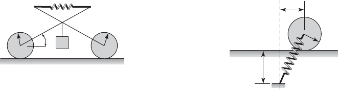
3.39 Use Lagrange's equation to derive the equation
describing the vibratory system shown in Figure
E3.39, which consists of two gears, each of radius r
and rotary inertia J. They drive an elastically con-
strained rack of mass m. The elasticity of the con-
straint is k. From the equation of motion, determine
an expression for the natural frequency.
3.40 Obtain the governing equation of motion in
terms of the generalized coordinate u for torsional
2z
c
mv
o
, and
U
o
U
l
t v
o
t, v
o
2
g
l
, Æ
v
v
o
,
d
2
u
dt
2
2z
du
dt
31 U
o
Æ
2
cos Æt 4sin u 0
cl
2
u
#
u1t 2 U cos vt
FIGURE E3.38
m
g
l
y
x
u(t)
cl
2
.
(t)
3.36 For the translating and rotating disc system of
Figure 3.9, choose the coordinate x measured from the
unstretched length of the spring to describe the mo-
tion of the system. What are the equivalent inertia,
equivalent stiffness, and equivalent damping proper-
ties for this system?
3.37 For the inverted pendulum system of Figure 3.10,
choose the coordinate x
1
measured from the un-
stretched length of the spring to describe the motion
of the system. What are the equivalent inertia, equiv-
alent stiffness, and equivalent damping properties for
this system?
3.38 Consider a pendulum with an oscillating support
as shown in Figure E3.38. The support is oscillating
harmonically at a frequency v; that is,
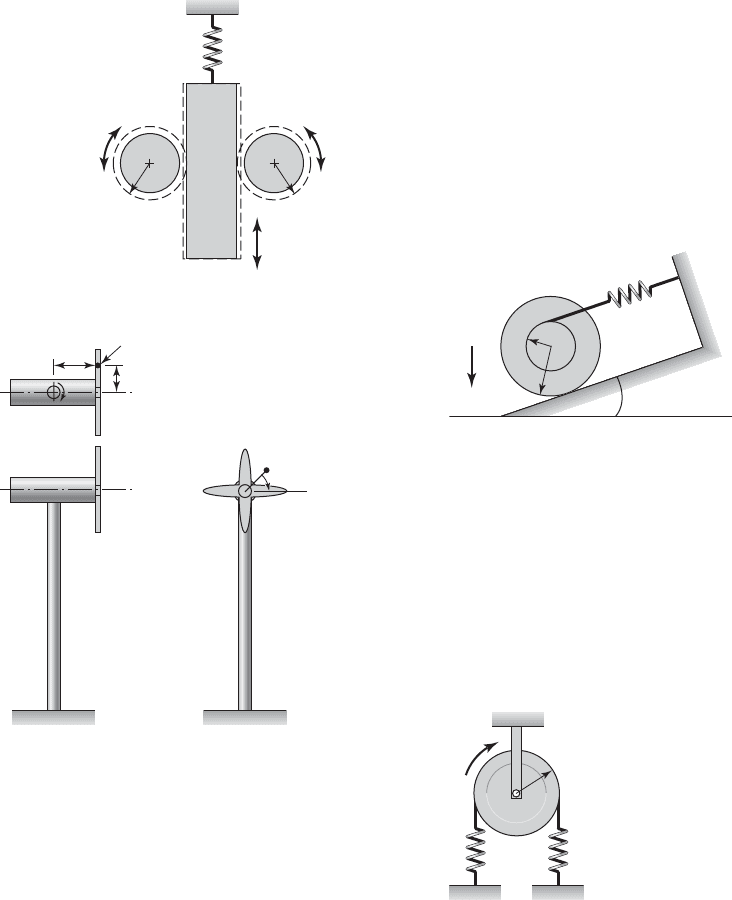
122 CHAPTER 3 Single Degree-of-Freedom Systems
Figure E3.41. The cylinder has another cylinder of ra-
dius r R concentrically attached to it. The smaller
cylinder has a cable wrapped around it. The other end
of the cable is fixed. The cable is parallel to the in-
clined surface. If the stiffness of the cable is k, the
mass and rotary inertia of the two attached cylinders
are m and J
O
, respectively, then determine an expres-
sion for the natural frequency of the system in Hz. The
length of the unstretched spring is L.
3.42 For the pulley shown in Figure E3.42, determine
an expression for natural frequency, for oscillations
about the static equilibrium position. The springs are
stretched by an amount x
o
at the static equilibrium.
The rotary inertia of the pulley about its center is J
O
,
the radius of the pulley is r, and the stiffness of each
translation spring is k.
oscillations of the wind turbine shown in Figure
E3.40. Assume that the turbine blades spin at v rad/s
and that the total mass unbalance is represented by
mass m
o
located at a distance e from the axis of rota-
tion. The support for the turbine is a solid circular rod
of diameter d, length L, and it is made from a material
with a shear modulus G. The turbine body and blades
have a rotary inertia J
z
. Assume that the damping co-
efficient for torsional oscillations is c
t
.
3.41 The uniform concentric cylinder of radius R rolls
without slipping on the inclined surface as shown in
FIGURE E3.40
L
k
t
, c
t
m
o
m
o
(t)
t
FIGURE E3.42
kk
r
J
O
O
FIGURE E3.41
k
m, J
O
R
a
r
O
g
FIGURE E3.39
k
x
rr
JJ
m
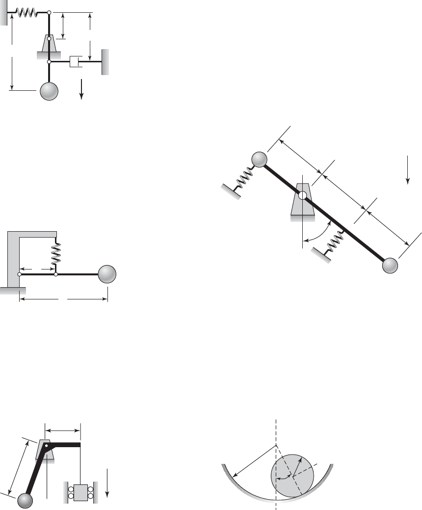
3.43 The pendulum shown in Figure E3.43 oscillates
about the pivot at O. If the mass of the rigid bar of
length L
3
can be neglected, then determine an expres-
sion for the damped natural frequency of the system
for “small” angular oscillations.
Exercises 123
3.44
Consider the pendulum shown in Figure E3.44. If
the bar is rigid and weightless, then determine the
natural frequency of the system and compare it to the
natural frequency of the pendulum shown in Figure
2.18b. What conclusions can you draw?
FIGURE E3.44
m
b
k
L
FIGURE E3.43
g
m
c
O
k
L
2
L
1
L
3
equilibrium as shown in the figure. For “small” angles
of rotation u about the static equilibrium position u
o
,
obtain an expression for the period.
3.46 For “small” oscillations u about the nominal po-
sition specified by the angle b, determine an expres-
sion for the natural frequency of the system shown in
Figure E3.46. The springs are not stretched in this
nominal position.
FIGURE E3.45
m
g
L
R
u
o
m
FIGURE E3.47
θ
ϕ
m
R
r
FIGURE E3.46
g
k
2
β
k
1
L
L
L
m
1
m
2
3.45 Consider the weightless rigid rod shown in Fig-
ure E3.45. At one end of the rod is a mass m, and from
the other end of the rod another mass m is suspended
from a taut string. The system is undamped and it is in
3.47 A circular cylinder of mass m and radius r rolls
on the interior of a cylindrical surface of radius R,as
shown in Figure E3.47. The system is in equilibrium
at u 0. Determine an expression for the natural fre-
quency of the system for “small” oscillations about
this equilibrium position.
124 CHAPTER 3 Single Degree-of-Freedom Systems
3.48
The undamped pendulum pivoted at point O
shown in Figure E3.48 has a cylinder of mass m
2
at its
top that rotates without slipping on the interior of
a cylinder. At the bottom end of the pendulum, a
mass m
1
is attached. The rod connecting the two
masses is rigid and weightless. The system is in
equilibrium at u 0. Determine an expression for the
period of oscillation of the system. Assume that
m
2
L
2
m
1
L
1
.
along the exterior surface of a cylinder. Determine the
equation of motion and obtain an expression for the
natural frequency of the system.
3.50 A floating rectangular prismatic bar with of spe-
cific gravity g is hinged at the water line as shown in
Figure E3.50. The thickness of the bar is b and the
mass density of the fluid is r. Determine the equation
of motion and obtain an expression for the natural fre-
quency of the system for “small” oscillations about
point O.
3.49 A rod of mass m pivots at point O, as shown in
Figure E3.49. Attached to the free end of the rod of
length R r is a mass M that rotates without slipping
3.51 For small oscillations, determine the equation of
motion and the natural frequency of the rotating pen-
dulum shown in Figure E3.51 that oscillates about the
equilibrium position b when the angular rotation is Æ.
FIGURE E3.49
ϕ
θ
m
M
r
O
R
FIGURE E3.50
L
L
1
βL
O
h
s
γ h
ρ
L
2
(1 β )L
h
x
z
c.g.
FIGURE E3.51
O
R
L
β
Ω
m
FIGURE E3.48
L
2
L
1
r
2
m
2
O
θ
ϕ
r
1
m
1
3.52 Determine the equation of motion and obtain the
natural frequency of the system shown in Figure
E3.52. The connecting rods are rigid and weightless.
Each of the wheels of radius r has a rotational inertia
J
o
and they roll without slipping.
Exercises 125
3.53
Obtain the equation of motion for the system
shown in Example 3.12 when the oscillations about
its upright position are no longer “small.”
3.54 A cylindrical disk of mass m and radius r rolls on
a surface without slipping, as shown in Figure E3.54.
The free length of the spring L is such that
Derive the governing equation of motion. Do not
make any assumptions about the magnitude of
oscillations.
L h r.
FIGURE E3.52
β
L
1
J
o
J
o
r
r
k
L
1
m
L
2
L
2
FIGURE E3.54
x
h
k
r
126
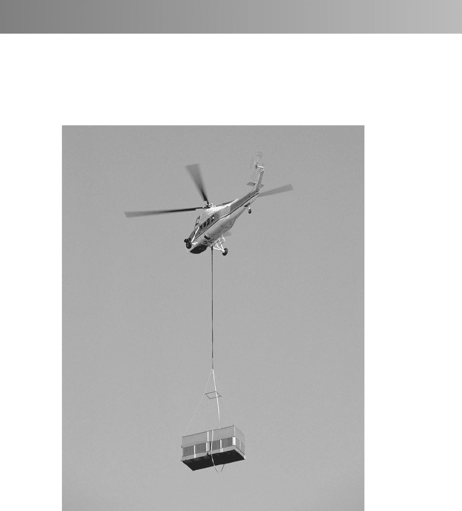
Free oscillations of systems are important considerations that must be taken into account in order to obtain effective operations of
a system. For a helicopter or a ship crane, the load oscillations must be taken into account to carry out safe load-transfer operations.
Stability of vibratory systems such as the machine tool must also be considered in the design of systems subjected to dynamic loads.
(Source: David Buttington /Getty Images.)

127127
4
Single Degree-of-Freedom System:
Free-Response Characteristics
4.1 INTRODUCTION
4.2 FREE RESPONSES OF UNDAMPED AND DAMPED SYSTEMS
4.2.1 Introduction
4.2.2 Initial Velocity
4.2.3 Initial Displacement
4.2.4 Initial Displacement and Initial Velocity
4.3 STABILITY OF A SINGLE DEGREE-OF-FREEDOM SYSTEM
4.4 MACHINE TOOL CHATTER
4.5 SINGLE DEGREE-OF-FREEDOM SYSTEMS WITH
NONLINEAR ELEMENTS
4.5.1 Nonlinear Stiffness
4.5.2 Nonlinear Damping
4.6 SUMMARY
EXERCISES
4.1 INTRODUCTION
In Chapter 3, we illustrated how the governing equation of a single degree-of-
freedom system can be derived. In this chapter, the solution of this governing
equation is determined, and based on this solution, the responses of single
degree-of-freedom systems subjected to different types of initial conditions
are discussed. As pointed out in Chapter 3, it is shown that the free responses
can be characterized in terms of the damping factor. The notion of stability of
a solution is introduced and briefly discussed. The problem of machine-tool

chatter during turning operations is also considered and numerical determi-
nation of stability for this problem is illustrated. The forced responses of sin-
gle degree-of-freedom systems are addressed in Chapters 5 and 6.
For all linear single degree-of-freedom systems, the governing equation
can be put in the form of Eq. (3.22), which is repeated below.
(4.1)
A solution is sought for the system described by Eq. (4.1) for a given set
of initial conditions. This type of problem is called an initial-value problem.
Since the system inertia, stiffness, and damping parameters are constant with
respect to time, the coefficients in Eq. (4.1) are constant with respect to time.
For such linear differential systems with constant coefficients, the solution
can be determined by using time-domain methods and the Laplace transform
method
1
, as illustrated in Appendix D. The latter has been used here, since a
general solution for the response of a forced vibratory system can be deter-
mined for arbitrary forms of forcing. However, a price that one pays for gen-
erality is that in the Laplace transform method the oscillatory characteristics
of the vibratory system are not readily apparent until the final solution is de-
termined. On the other hand, when time-domain methods are used, the ex-
plicit forms of the solutions assumed in the initial development allows one to
readily see the oscillatory characteristics of a vibratory system. In order to
provide a flavor of this complementary approach, time-domain methods are
summarized in Appendix D.
The ease with which we can use Laplace transforms to solve linear, ordi-
nary differential equations is illustrated by solving for the response of a sys-
tem with a Maxwell material later in the chapter and by solving for the re-
sponse of a two degree-of-freedom system in Chapter 8. We also show how
to use Laplace transforms to solve for the free responses of thin beams in
Chapter 9. An advantage of using the Laplace transform approach is the con-
venience with which one can see the duality of the responses in the time do-
main and the frequency domain; this is important for understanding how the
same information can be expressed in the two different domains.
In this chapter, we shall show how to:
• Determine the solutions for a linear, single degree-of-freedom system that
is underdamped, critically damped, overdamped, and undamped.
• Determine the response of single degree-of-freedom systems to initial con-
ditions and use the results to study the response to impact and collision.
• Determine when a system is stable and how to use the root-locus diagram
to obtain stability information.
• Obtain the conditions under which a machine tool chatters.
• Use different models for damping: viscous (Voigt), Maxwell, hysteretic.
• Examine systems with nonlinear stiffness and nonlinear damping.
d
2
x
dt
2
2zv
n
dx
dt
v
2
n
x
f 1t 2
m
128 CHAPTER 4 Single Degree-of-Freedom System
1
See Appendix A.

4.2 FREE RESPONSES OF UNDAMPED AND DAMPED SYSTEMS
4.2.1 Introduction
In this section, the responses of undamped and damped single degree-of-
freedom systems in the absence of forcing—that is, f(t) 0—are explored in
detail. These responses are also referred to as free responses, and when the
system is undamped or underdamped, the responses are referred to as free os-
cillations. In the absence of forcing, the single degree-of-freedom given by
Eq. (4.1) reduces to
(4.2)
Free responses are the responses of a system to either an initial displace-
ment x(t) X
o
, an initial velocity , or to both an initial displace-
ment and an initial velocity. Based on the discussion in Appendix D, there are
four distinct types of solutions to Eq. (4.1) depending on the magnitude of the
damping factor z. These four regions describe four different types of systems
as follows.
Underdamped System: 0 z 1
When the damping factor is in the range 0 z 1, we denote the system as
an underdamped system. From Eq. (3.20), we see that in this region, the
damping coefficient c is less than the critical damping coefficient c
c
. For val-
ues of z in this range, the solutions to Eq. (4.2) are given by either Eq. (D.15)
or Eq. (D.16); that is,
(4.3)
or
(4.4)
respectively, where
(4.5)
where v
d
is the damped natural frequency and
(4.6)w
d
tan
1
v
d
X
o
V
o
zv
n
X
o
A
o
B
X
o
2
a
V
o
zv
n
X
o
v
d
b
2
v
d
v
n
21 z
2
x1t 2 A
o
e
zv
n
t
sin1v
d
t w
d
2
x1t 2 X
o
e
zv
n
t
cos1v
d
t2
V
o
zv
n
X
o
v
d
e
zv
n
t
sin1v
d
t2
x
#
10 2 V
o
d
2
x
dt
2
2zv
n
dx
dt
v
2
n
x 0
4.2 Free Responses of Undamped and Damped Systems 129