Balakumar Balachandran, Magrab E.B. Vibrations
Подождите немного. Документ загружается.

Upon using Laplace transform pairs 14 and 16 in Table A of Appendix A,
the inverse Laplace transform of Eq. (o) results in Eq. (4.23). The numeri-
cally
4
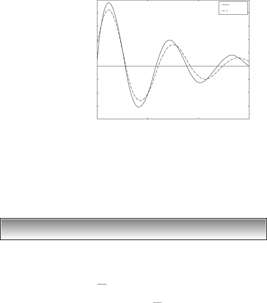
computed inverse Laplace transforms of Eq. (n) for z 0.15 and
g 1 and Eq. (o) for z 0.15 are shown in Figure 4.12. At t 0, we see
that the reaction force F
B
has a discontinuity for the Kevin-Voigt model, while
this reaction force is zero for the Maxwell model.
EXAMPLE 4.8
Vibratory system with Maxwell model revisited
As a continuation of Example 4.7, we now consider the case where the sup-
port consists only of a Maxwell element; that is, the spring k is absent. In this
case, we again examine the force transmitted to the fixed base. Setting k 0
in Eq. (a) of Example 4.7, we arrive at
(a)k
1
1x x
d
2 c
dx
d
dt
m
d
2
x
dt
2
k
1
1x x
d
2 f 1t 2
150 CHAPTER 4 Single Degree-of-Freedom System
FIGURE 4.12
Reaction force of the system shown in Figure 4.11 for z 0.15.
1
0.8
0.6
0.4
0.2
0
0.2
0.4
0.6
0.8
0 5 10 15
F
B
/(kV
o
/v
n
)
t
g
1
g
→ ∞
4
The MATLAB function ilaplace from the Symbolic Toolbox was used.

Introducing a new set of quantities
and (b)
Eq. (a) is written as
(c)
where the overdot now indicates the derivative with respect to t and
(d)
If we represent the Laplace transform of x(t) by X(s), the Laplace trans-
form of x
d
(t) by X
d
(s), and the Laplace transform of f(t) by F(s), then, from
pair 2 in Table A of Appendix A, the Laplace transforms of Eqs. (c) are
(e)
where we have assumed that x
d
(0) 0 and
(f)
Upon solving for X(s) and X
d
(s) in Eqs. (e), we obtain
(g)
where
(h)
Note that z
m
1 only when z
1
0.25.
When the spring with stiffness k is absent, the reaction force on the base is
(i)
which is rewritten in terms of the nondimensional quantity given by Eq. (b) as
(j)
F
B
1t¿ 2
k
1
2z
1
x
#
d
F
B
1t 2 F
1
c
dx
d
dt
2z
m
1
2z
1
k
1
cv
1n
X
d
1s 2
G
1
1s 2
s12z
1
s
2
s 2z
1
2
X1s 2
G
1
1s 211 2z
1
s2
s12z
1
s
2
s 2z
1
2
G
1
1s 212z
m
s2
s1s
2
2z
m
s 12
G
1
1s 2
F1s 2
k
1
sx10 2 x
#
10 2
X1s 2 11 2z
1
s2X
d
1s 2 0
1s
2
12X1s 2 X
d
1s 2 G
1
1s 2
2z
1
cv
1n
k
1
x x
d
2z
1
x
#
d
x
$
x x
d
f 1t 2/k
1
v
1
2
n
k
1
m
t¿ v
1n
t
4.2 Free Responses of Undamped and Damped Systems 151

where the overdot is the derivative with respect to t. Upon taking the Laplace
transform of Eq. (j), assuming that x
d
(0) 0, and using the second of Eqs.
(g), we find that
(k)
We again limit the discussion to the case where the applied force and the
initial displacement are zero; that is, f(t) 0 and x(0) 0, and the initial ve-
locity is
(l)
Therefore, Eq. (f) simplifies to
(m)
Upon substituting Eq. (m) into Eq. (k), we arrive at
(n)
For z
m
1, the inverse Laplace transform of Eq. (n) is given by Laplace trans-
form pair 15 in Table A of Appendix A with v
n
1 and z z
m
. The numer-
ically computed
5
inverse Laplace transform of Eq. (n) for z
m
0.15 and
z
m
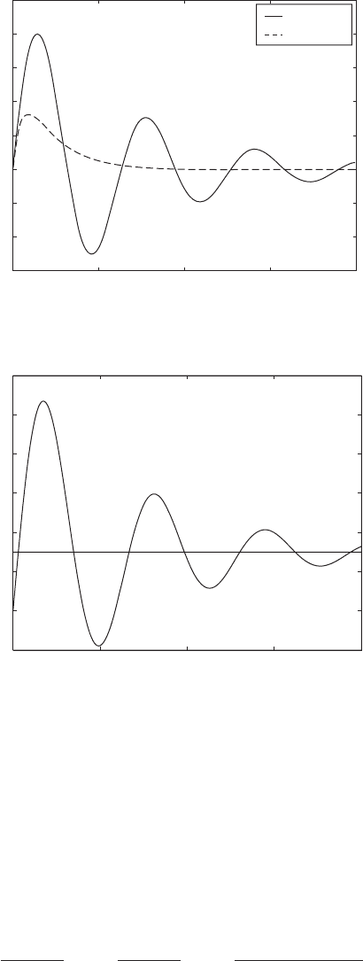
1.2 are shown in Figure 4.13a. This model also exhibits a reaction force
F
B
0 at t0. The limiting value of this force is determined from trans-
form pair 31 in Table A of Appendix A as
(o)
In Figure 4.13b, we have plotted the displacement response obtained
from the numerical inverse Laplace transform of the first of Eqs. (g) with
G
1
(s) given by Eq. (m) and for z
m
0.15. It is noticed that the nondimen-
sional displacement ratio does not approach zero as time increases. This is be-
cause there is no spring in parallel with the viscous damper to restore the sys-
tem to its original equilibrium position and, therefore, the Maxwell element
undergoes a permanent deformation. Consequently, based on these observa-
lim
t¿씮 q
F
B
1t¿ 2
1k
1
V
o
/v
1n
2
씮 lim
s씮 0
sF
B
1s 2
1k
1
V
o
/v
1n
2
lim
s씮 0
s
1s
2
2z
m
s 12
0
1
1s
2
2z
m
s 12
F
B
1s 2
1k
1
V
o
/v
1n
2
2z
1
12z
1
s
2
s 2z
1
2
G
1
1s 2
V
o
v
1n
dx10 2
dt
v
1n
dx10 2
dt¿
V
o
F
B
1s 2
k
1
2z
1
G
1
1s 2
12z
1
s
2
s 2z
1
2
152 CHAPTER 4 Single Degree-of-Freedom System
5
The function ilaplace from MATLAB’s Symbolic Toolbox was used.
tions, the Maxwell model is not used by itself, but in parallel with another
spring, as shown in Figure 4.11. The limiting value is determined from trans-
form pair 31 in Table A of Appendix A as
(p)lim
t¿씮 q
x1t¿ 2
1V
o
/v
1n
2
씮 lim
s씮 0
sX1s 2
1V
o
/v
1n
2
lim
s씮 0
s12z
m
s2
s1s
2
2z
m
s 12
2z
m
0.3
4.2 Free Responses of Undamped and Damped Systems 153
FIGURE 4.13
Maxwell element: (a) reaction force of the system for z
m
0.15 and z
m
1.2, and (b) dis-
placement response of the mass for z
m
0.15.
0 5 10 15 20
0.6
0.4
0.2
0
0.2
0.4
0.6
0.8
1
t
F
B
/(k
1
V
o
/v
1n
)
z
m
0.15
z
m
1.2
(a)
0 5 10 15 20
0.2
0
0.2
0.4
0.6
0.8
1
1.2
t
x(t
)/(V
o
/v
1n
)
(b)

4.2.3 Initial Displacement
We now examine the free response of an underdamped single degree-of-
freedom system with a prescribed initial displacement. When a system is
subjected to an initial displacement only, we set V
o
0 and Eq. (4.6) for the
amplitude and phase simplify to
Therefore, Eq. (4.4), which describes the displacement response, becomes
(4.28)
and, after using Eq. (D.12), the velocity and acceleration are, respectively,
(4.29)
Equations (4.28) and (4.29) are plotted in Figure 4.14 and the correspon-
ding state space plot is shown in Figure 4.15 along with their respective time
histories. As time unfolds, the trajectory is attracted to the equilibrium posi-
tion located at the origin (0, 0).
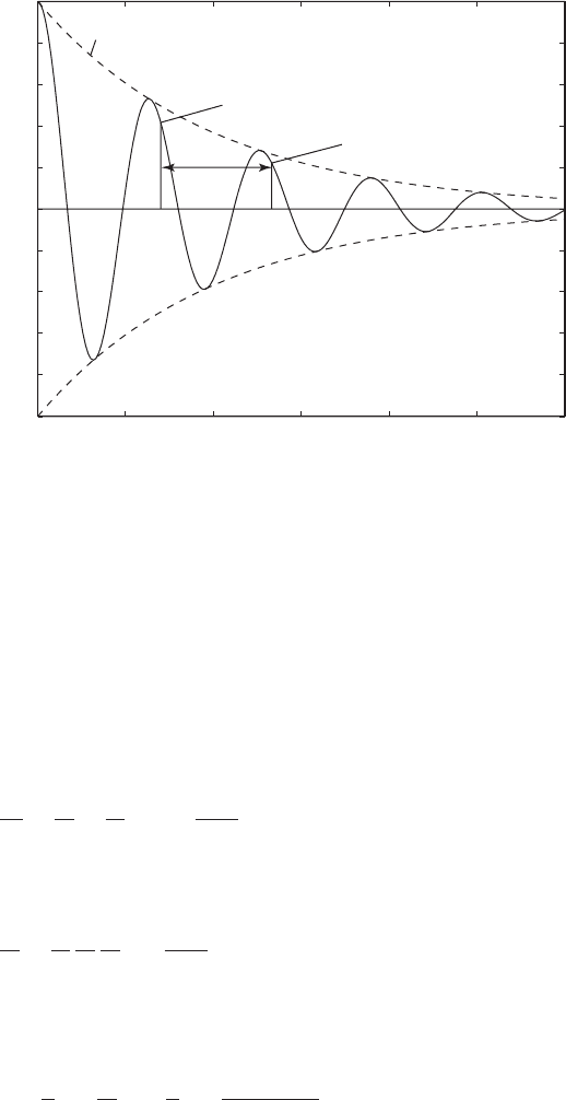
Logarithmic Decrement
6
Consider the displacement response of a single degree-of-freedom system
subjected to an initial displacement as shown in Figure 4.16. The logarithmic
decrement d is defined as the natural logarithm of the ratio of any two suc-
cessive amplitudes of the response that occur a period T
d
apart, where T
d
is
given by
(4.30)
From these two amplitudes, it is possible to determine the damping
ratio z. To this end, we determine a relationship between the logarithmic
decrement and the damping factor. We start from
(4.31)d ln a
x1t 2
x1t T
d
2
b
T
d
2p
v
d
2p
v
n
21 z
2
x
$
1t 2 a1t2
X
o
v
n
2
21 z
2
e
zv
n
t
sin1v
d
t w2
x
#
1t 2 v1t2
X
o
v
n
21 z
2
e
zv
n
t
sin1v
d
t2
x1t 2
X
o
21 z
2
e
zv
n
t
sin1v
d
t w2
w
d
tan
1
21 z
2
z
w
A
o
X
o
21 z
2
154 CHAPTER 4 Single Degree-of-Freedom System
6
Although the definition of the logarithmic decrement is provided in Section 4.2.3, it applies
equally to all free responses considered in Section 4.2.
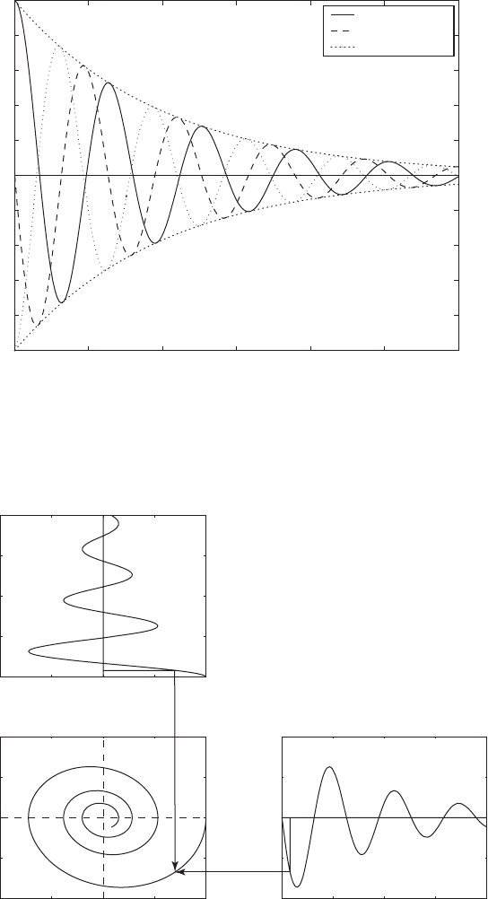
FIGURE 4.14
Time histories of displacement, velocity, and acceleration of a system with a prescribed initial
displacement.
FIGURE 4.15
State-space plot of single degree-of-freedom system with prescribed initial displacement.
0 5 10 15 20 25 30
1
0.8
0.6
0.4
0.2
0
0.2
0.4
0.6
0.8
1
v
n
t
x(t)/X
o
, v(t)/(X
o
v
n
), a(t)/(X
o
v
n
2
)
e
zv
n
t
Displacement
Velocity
Acceleration
1
0.5 0 0.5 1
1
0.5 0 0.5 1
0
5
10
15
20
t
1
v
n
t
x(t)/X
o
1
1
0.5
0.5
0
0.5
1
x(t)/X
o
v(t)/(X
o
v
n
)
0 5 10 15 20
0
0.5
1
t
1
v
n
t
v(t)/(X
o
v
n
)
If we let
(4.32)
then, by definition,
(4.33)
Furthermore, we also notice from Eq. (4.33) that
and, therefore, the logarithmic decrement in terms of two amplitudes mea-
sured p cycles apart is expressed as
(4.34)
Making use of Eq. (4.28) and Eq. (4.30) and substituting for the free re-
sponse p cycles apart into Eq. (4.34), we obtain
d
1
p
ln
a
x
o
x
p
b
1
p
ln
a
x1t 2
x1t pT
d
2
b
p 1, 2, . . .
x
0
x
p
x
0
x
1
x
1
x
2
x
2
x
3
###
x
p 1
x
p
e
pd
x
0
x
1
x
1
x
2
x
2
x
3
###
x
p 1
x
p
e
d
x
p
x1t pT
d
2
p 0, 1, 2, . . .
156 CHAPTER 4 Single Degree-of-Freedom System
FIGURE 4.16
Quantities used in the definition of the logarithmic decrement.
0 5 10 15 20 25 30
1
0.8
0.6
0.4
0.2
0
0.2
0.4
0.6
0.8
1
x(t)/
X
o
x(t
T
d
)/X
o
v
n
T
d
v
n
T
d
2p/(1
z
2
)
1/2
v
n
t
x(t)/X
o
e
zv
n
t
(4.35)
Thus, from a measurement of the amplitudes x
0
and x
p
, one can obtain the
damping ratio z from
(4.36)
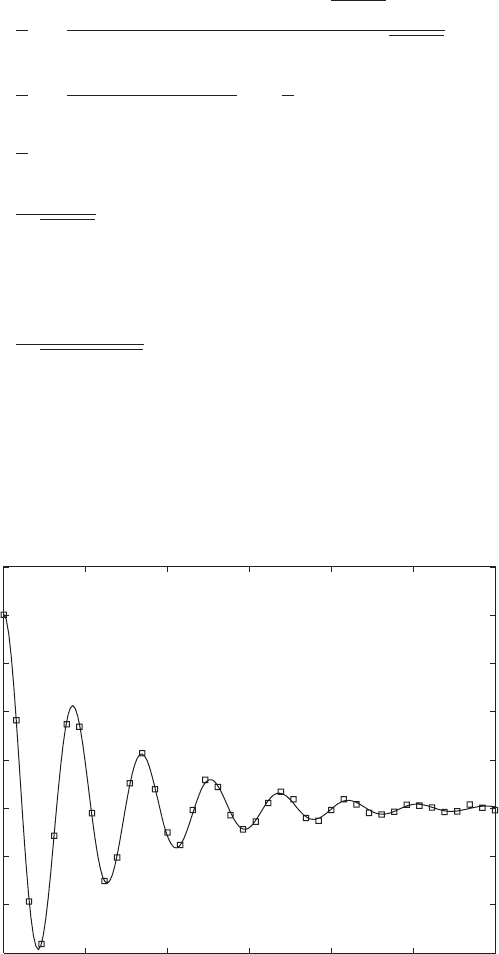
As an alternative to this type of estimation for d, the free response of a
system can also be curve-fitted to determine the damping factor. Based on
digitally sampled data, one can use a standard nonlinear curve-fitting proce-
dure for estimating the amplitude, damping ratio, and natural frequency of a
system based on Eq. (4.28). A representative set of sampled data and the nu-
merically obtained curve-fit values
7
are shown in Figure 4.17. The open
z
1
21 12p/d2
2
2pz
21 z
2
1
p
zv
n
pT
d
zv
n
T
d
1
p
ln
a
e
zv
n
pT
d
sin1v
d
t w2
sin1v
d
t w 2pp 2
b
1
p
ln
1e
zv
n
pT
d
2
d
1
p
ln
a
X
o
e
zv
n
t
sin1v
d
t w2/ 21 z
2
X
o
e
zv
n
1t pT
d
2
sin1v
d
1t pT
d
2 w2/ 21 z
2
b
4.2 Free Responses of Undamped and Damped Systems 157
7
These results were obtained using lsqcurvefit from the MATLAB Optimization Toolbox.
FIGURE 4.17
Curve fit to a set of sampled data from the response of a system with prescribed initial
displacement.
0 5 10 15 20 25 30
0.6
0.4
0.2
0
0.2
0.4
0.6
0.8
1
t
Amplitude
Fitted values
z
0.101
v
n
1.5 rad/s
X
o
0.803 units

squares represent the data through which the fitted curve is depicted as a solid
line. As discussed in Section 5.3.2, the estimation of parameters such as
damping factor and natural frequency can be also carried out based on the sys-
tem transfer function.
EXAMPLE 4.9
Estimate of damping ratio using the logarithmic decrement
It is found from a plot of the response of a single degree-of-freedom system
to an initial displacement that at time t
o
the amplitude is 40% of its initial
value. Two periods later the amplitude is 10% of its initial value. We shall de-
termine an estimate of the damping ratio. Thus, from Eq. (4.34)
Then, from Eq. (4.36), we find that
4.2.4 Initial Displacement and Initial Velocity
We shall now consider the case when a system is subjected to an initial dis-
placement and an initial velocity simultaneously. The solution is given by
Eq. (4.4), which is repeated below for convenience.
(4.37)
From Eqs. (4.6), we find that the amplitude and phase are given by
(4.38)
and V
r
V
o
/(v
n
X
o
) is a velocity ratio. The velocity response is determined
from Eq. (4.37) to be
(4.39)
where w is given by Eq. (4.15).
The numerically evaluated result for x(t)/X
o
is shown in Figure 4.18. For
“small” values of V
r
, the displacement response is similar to that obtained for
a system with a prescribed initial displacement and for “large” values of V
r
,
the displacement response is similar to that obtained for a system with a pre-
scribed initial velocity.
x
#
1t 2A
o
v
n
e
zv
n
t
sin1v
d
t w
d
w2
w
d
tan
1
v
d
X
o
V
o
zv
n
X
o
tan
1
21 z
2
z V
r
A
o
B
X
o
2
a
V
o
zv
n
X
o
v
d
b
2
X
o
B
1
1V
r
z2
2
1 z
2
x1t 2 A
o
e
zv
n
t
sin1v
d
t w
d
2
z
1
21 12p/0.6932
2
0.11
d
1
2
ln a
0.4
0.1
b 0.693
158 CHAPTER 4 Single Degree-of-Freedom System
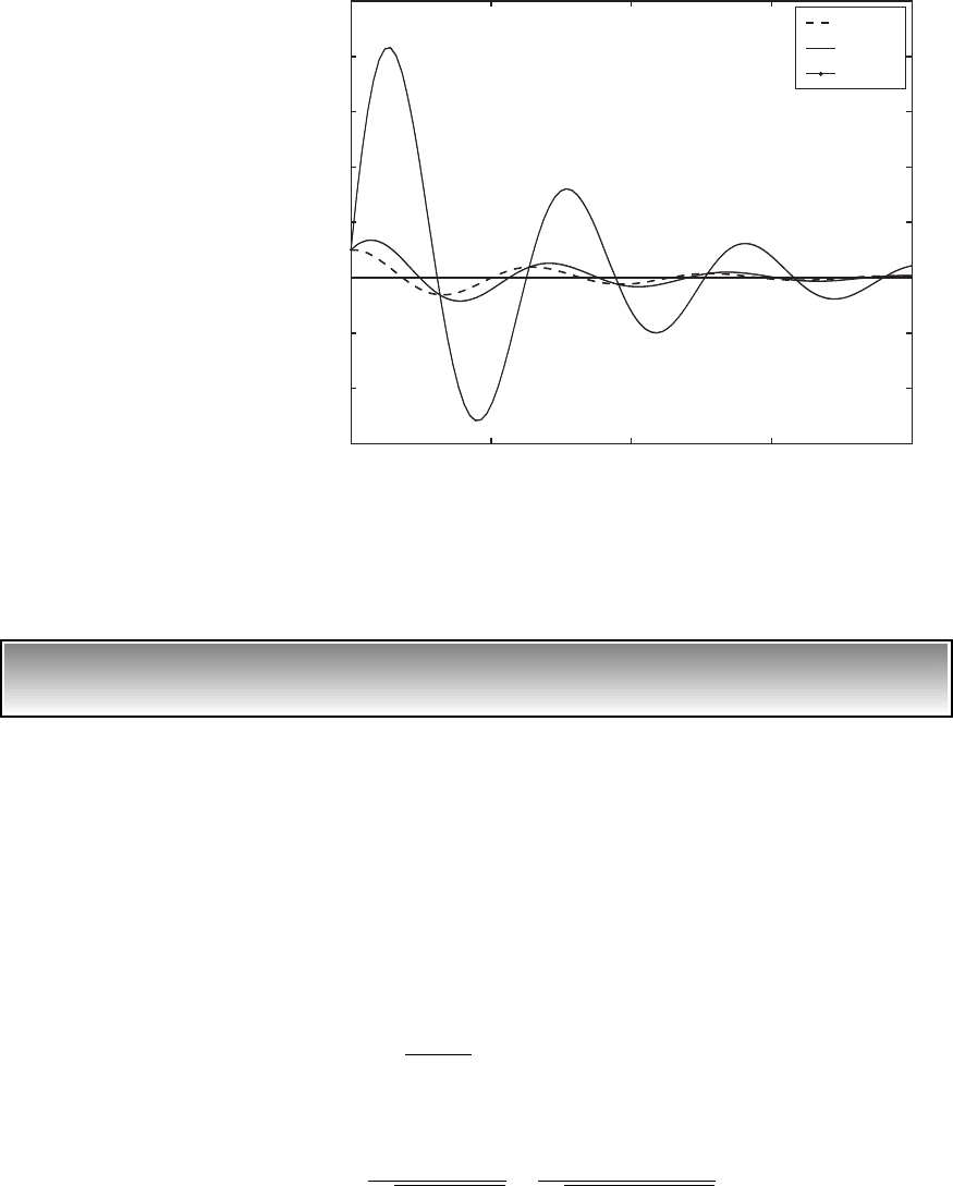
EXAMPLE 4.10 Inverse problem: information from a state-space plot
Consider the state-space plot shown in Figure 4.19. From this graph, we shall
determine the following: (a) the value of the damping ratio and (b) the time
t
max
v
n
t
max
at which the maximum displacement occurs.
From the graph, the initial conditions are x(0) X
o
and v(0) 1.6X
o
v
n
.
To determine z, the logarithmic decrement is used. For convenience, we
select the values of the displacement from Figure 4.19 that are along the line
v(t) 0. Then,
and (a)
and from Eq. (4.34) and Eq. (a), we determine the logarithmic decrement
(b)
Then, from Eq. (4.36) and Eq. (b), we find the damping factor to be
(c)z
1
21 12p/d2
2
1
21 12p/0.6422
2
0.10
d ln a
0.95 X
o
0.5X
o
b ln11.902 0.642
x1t T
d
2 0.5 X
o
x1t 2 0.95X
o
4.2 Free Responses of Undamped and Damped Systems 159
FIGURE 4.18
Displacement response of a system with prescribed initial displacement and prescribed
initial velocity.
0 5 10 15 20
6
4
2
0
2
4
6
8
10
v
n
t
x(t)/X
o
V
r
0.1
V
r
1
V
r
10