Balakumar Balachandran, Magrab E.B. Vibrations

Подождите немного. Документ загружается.

0 2 4 6 8 10 12



0.1

0.05

0.1

(a)

0 2 4 6 8 10 12



0.1



0.05

(t)

(b)



0.05

(t)

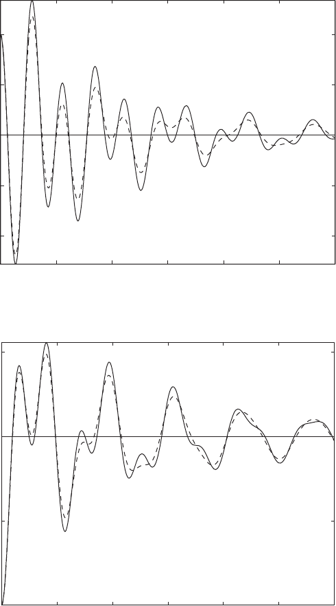
FIGURE 8.7

Displacements of a two degree-of-freedom system with two different damping models when

both masses are subjected to equal, but opposite, initial displacements: (a) displacement of

and (b) displacement of m

. Solid lines correspond to the constant damping model of Ex-

ample 8.2 with z  0.05 and dashed lines correspond to an arbitrary damping model whose

damping matrix is given by Eq. (g).

which is not a diagonal matrix. In this case, the matrix given by Eq. (g) is

used along with the matrices and from Eqs. (a) of Example 7.20 to

form the matrices and in Eqs. (8.58). These matrices are used, in turn,

in Eq. (8.56) to numerically obtain the state vector {Y}. The results for the dis-

placement states are shown in Figure 8.7.

On comparing the results of Figure 8.7, it is seen that there are discernible

differences between the free oscillations of the two cases in which the only dif-

ference between the models of the two systems is due to the damping matrix.

8.4

LAPLACE TRANSFORM APPROACH

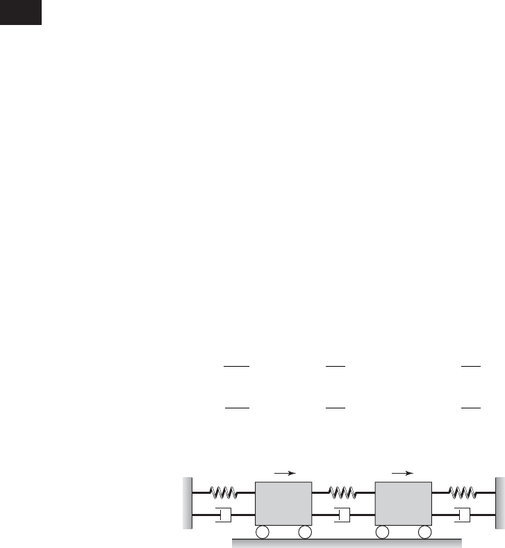
In this section, the general solution for the response of a system such as that

shown in Figure 8.8 is determined by using Laplace transforms. This method

is applicable to linear systems of differential equations with constant coefﬁ-

cients, either in the second-order form of Eq. (7.3) or in the ﬁrst-order form

of Eq. (8.56). The procedure to determine the solution follows along the lines

of what was illustrated in Appendix D for single degree-of-freedom systems.

First, the governing system of differential equations is transformed into an al-

gebraic system of equations by using Laplace transforms. Next, we solve this

algebraic system to determine the responses of the different inertial elements

in the Laplace domain. In the ﬁnal step, these responses are transformed back

to the time domain by using the inverse Laplace transform. As had been done

in Chapter 4, this ﬁnal step is not explicitly carried out here. Instead, we ei-

ther take recourse to tables such as those presented in Appendix A or numer-

ically evaluate the quantities with the appropriate MATLAB functions.

For purposes of illustration and algebraic ease, the discussion is re-

stricted to two degree-of-freedom systems. The governing equations of mo-

tion of the system shown in Figure 8.8 are given by Eq. (7.1b), which are re-

peated below.

(8.60) m

 1c

 c

 1k

 k

 c

 k

 f

1t 2

 1c

 c

 1k

 k

 c

 k

 f

1t 2

3B 43A 4

3K 43M 4

3C 4

8.4 Laplace Transform Approach 471

, f

(t) x

, f

(t)

FIGURE 8.8

System with two degrees of freedom.

Introducing the nondimensional quantities from Eqs. (7.41) and the following

additional quantities for the nondimensional time, damping factor, and damp-

ing coefﬁcient ratio, respectively,

(8.61)

Eqs. (8.60) are rewritten as

(8.62)

Carrying out the Laplace transforms of the different terms on each side

of Eqs. (8.62) and making use of Laplace transform pair 2 in Table A of

Appendix A, we arrive at

(8.63)

where the coefﬁcients A(s), B(s), C(s), and E(s) are given by

(8.64)

and

(8.65)

In Eqs. (8.65), the transforms K

(s) and K

(s) are determined by the forcing

and the initial conditions, the overdot indicates the time derivative with re-

spect to the nondimensional time t, X

(s) and X

(s) are the Laplace transforms

of x

(t) and x

(t), respectively, and F

(s) and F

(s) are the Laplace transforms

of the force inputs, f

(t) and f

(t), respectively. Furthermore, x

(0) and (0)

are the initial displacement and the initial velocity of mass m

, respectively,

and x

(0) and are the initial displacement and the initial velocity of mass

, respectively.

10 2

1s 2

1s 2

 x

10 2 3s  2z

11  c

24x

10 2 2z

10 2

1s 2

1s 2

 x

10 2 3s  2z

 2z

10 2 2z

10 2

E1s2 s

 2z

11  c

2s  v

11  k

C1s 2 B1s 2/m

 2z

s  v

B1s 2 2z

s  m

A1s 2 s

 21z

 z

2s  1  m

C1s 2X

1s 2 E1s2X

1s 2 K

1s 2

A1s2X

1s 2 B1s2X

1s 2 K

1s 2

 v

11  k

 2z

 v



1t 2

 2z

11  c

 11  m

 2z

 m



1t 2

 12z

 2z

t  v



and



472 CHAPTER 8 Multiple Degree-of-Freedom Systems

Solving for X

(s) and X

(s) from Eqs. (8.63) yields

(8.66)

where the denominator D

(s) is given by

(8.67)

From Eq. (8.67), we can obtain the characteristic equation associated

with free oscillations of a two degree-of-freedom system by setting the damp-

ing factors z

 z

 0 and s  j. This results in the characteristic equation,

Eq. (7.45), which was obtained in the context of free oscillations of the un-

damped system.

The desired displacement responses x

(t) and x

(t) are determined by ex-

ecuting the inverse Laplace transforms of X

(s) and X

(s) given by Eqs. (8.66).

The solution

(8.68)

is referred to as the general solution for the response of the two degree-of-

freedom system given by Eqs. (8.62). The symbol L

1

denotes the inverse

Laplace transform. To determine the inverse Laplace transforms in Eqs.

(8.68), the method of partial fractions and the table provided in Appendix A

can be used. Alternatively, readily available algorithms such as the ones in the

MATLAB Controls Toolbox and Symbolic Math Toolbox can be used to de-

termine the responses based on Eqs. (8.66). In the next two sections, we il-

lustrate how the responses can be determined for arbitrary forcing and arbi-

trary initial conditions.

8.4.1 Response to Arbitrary Forcing

If we assume that the initial conditions are zero and that we have arbitrary

forcing, the transforms K

(s) and K

(s) in Eqs. (8.65) reduce to

(8.69)

where F

(s) is the Laplace transform of the force input f

(t). We now consider

two cases of forcing.

1s 2

1s 2

1s 2

1s 2

1t 2 L

1

1s 24

for

j  1, 2

 v

31  k

11  m

 32z

 2z

 2k

 z

2 2c

11  m

24s

 31  m

 v

 4z

 v

 4z

 z

24s

1s 2 s

 32z

 2z

11  c

24s

1s 2

1s 2C1s2

1s 2



1s 2A1s2

1s 2

1s 2

1s 2E1s2

1s 2



1s 2B1s2

1s 2

8.4 Laplace Transform Approach 473

Impulse Excitation

As a ﬁrst case, we determine the response of the vibratory system shown in

Figure 8.8, when the second mass is subjected to an impulse; that is,

(8.70)

Upon using the Laplace transform pair 5 in Table A of Appendix A, we de-

termine that

(8.71)

Then, from Eqs. (8.69), the transforms K

(s) and K

(s) are

(8.72)

Based on Eqs. (8.66) and (8.72), the displacement responses in the Laplace

domain are given by

(8.73)

For the special case where k

 c

 0 in Figure 8.8—that is k



 0—the polynomial D

(s) reduces to

(8.74)

and Eqs. (8.73) reduce to

(8.75)

Step Input

As a second case, we consider the determination of the response of the vibra-

tory system shown in Figure 8.8 when the second mass is subjected to a step

input; that is,

(8.76)

Upon using the Laplace transform pair 6 in Table A of Appendix A, we de-

termine that

(8.77)F

1s 2

1t 2 0

and

1t 2 F

u1t 2

1s 2

A1s 2

1s 2

1s 2

B1s 2

1s 2



C1s 2

1s 2

 32z

 2z

4s  v

1s 2 s

 32z

 2z

 31  m

 v

 4z

1s 2

A1s 2

1s 2

1s 2

B1s 2

1s 2



C1s 2

1s 2

1s 2

1s 2



1s 2

1s 2

 0

1s 2 F

1t 2 0

and

1t 2 F

d1t 2

474 CHAPTER 8 Multiple Degree-of-Freedom Systems

Then, from Eqs. (8.69), the transforms K

(s) and K

(s) are given by

(8.78)

Based on Eqs. (8.66) and (8.78), the displacement responses in the Laplace

domain are

(8.79)

For the special case where k

 c

 0 in Figure 8.8—that is k



 0—the polynomial D

(s) reduces to D

(s) given by Eq. (8.74) and the

responses given by Eqs. (8.79) reduce to

(8.80)

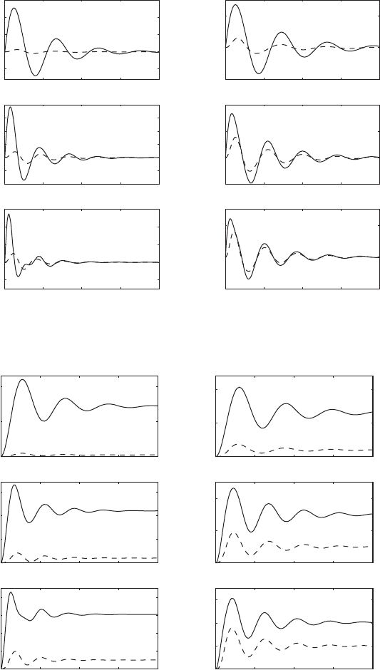
To determine the time-domain responses, the inverse Laplace transforms

of the impulse response given by Eqs. (8.75) and the step response given by

Eqs. (8.80) were evaluated numerically,

and the results obtained are shown

in Figures 8.9 and 8.10. In each of Figures 8.9 and 8.10, the response of the

mass m

is graphed by using a dashed line and the response of mass m

graphed by using a solid line. The response of the second mass is more pro-

nounced compared to the response of the ﬁrst mass, since the forcing is di-

rectly applied to the second mass. However, due to the coupling in the stiff-

ness and damping matrices, the mass m

also responds to the forcing. In the

case of the impulse excitation applied to the second mass, at the higher value

of the mass ratio m

, the responses of the ﬁrst and second masses are charac-

terized by damped oscillations with the same period for v

 1. In the case of

the step input, this observation is true of the transient oscillations. On exam-

ining Figure 8.10, it is seen that the settling positions of the two masses are

different for the given step input.

8.4.2 Response to Initial Conditions

We use the general solution given by Eqs. (8.66) to examine free oscillations of

the system shown in Figure 8.8 for different initial conditions. In order to iso-

late the response to initial conditions, we set the forcing f

(t) and f

(t)in

1s 2

A1s 2

1s 2

1s 2

B1s 2

1s 2



C1s 2

1s 2

1s 2

A1s 2

1s 2

1s 2

B1s 2

1s 2



C1s 2

1s 2

1s 2

1s 2 0

8.4 Laplace Transform Approach 475

The MATLAB functions tf, step, and impulse from the Controls Toolbox were used.

0 10 20 30 40







0.6 



0.6





1 







1.4 



1.4

0 10 20 30 40

1,2

()/(F

)

1,2

()/(F

)

0 10 20 30 40



0 10 20 30 40



0 10 20 30 40



0 10 20 30 40



(a) (b)



0 10 20 30 40

1,2

()/(F

)

1,2

()/(F

)

0 10 20 30 40



0 10 20 30 40



(a) (b)





0.6









1.4





0.6









1.4

FIGURE 8.9

Normalized displacement responses

of a two degree-of-freedom system

when m

is subjected to an impulse

force, z

 z

 0.2, k

 c

 0,

and t  v

t: (a) m

 0.1 and

(b) m

 0.5. [Dashed line x

(t);

solid line x

(t).]

FIGURE 8.10

Normalized displacement responses

of a two degree-of-freedom system

when m

is subjected to a step

force, z

 z

 0.2, k

 c

 0,

and t  v

t: (a) m

 0.1 and

(b) m

 0.5. [Dashed line x

(t);

solid line x

(t).]

Eqs. (8.62) to zero. Therefore, the corresponding Laplace transforms are F

(s)

 0 and F

(s)  0, and the transforms K

(s) and K

(s) in Eqs. (8.65) reduce to

(8.81)

For the special case where the spring k

and the damper c

are not present in

Figure 8.8—that is, k

 c

 0—the coefﬁcient E(s) in Eqs. (8.64) reduces to

(8.82)

and the function K

(s) in Eqs. (8.81) reduces to

(8.83)

The polynomial D

(s) in Eq. (8.67) reduces to the polynomial D

(s) given by

Eq. (8.74) and, therefore, the responses of the masses m

and m

given by Eqs.

(8.66) in the Laplace domain reduce to

(8.84)

where K

(s) is given by Eqs. (8.81), K

(s) is given by Eq. (8.83), E

(s) is

given by Eq. (8.82), D

(s) is given by Eq. (8.74), and A(s) and B(s) are given

by Eqs. (8.64).

We now consider the special case where the masses m

and m

in Fig-

ure 8.8 are both subjected to the same initial velocity V

; that is, the initial

conditions are

(8.85)

Noting from Eqs. (8.61) that the nondimensional time t  v

t, the transforms

(s) and K

(s) given by Eqs. (8.81) and (8.83), respectively, reduce to

(8.86)

and, therefore, Eqs. (8.84) reduce to

(8.87)

The time-domain responses x

(t) and x

(t) are the inverse transforms of

Eqs. (8.87). These have been obtained numerically

and they are shown in

Figure 8.11. In Figure 8.11, solid lines are used to depict the response of the

1s 2

1s 2

3C1s2 A1s 24

1s 2

1s 2

1s 2 B1s24

1s 2 x

10 2 V

1s 2 x

10 2 V

10 2 0,

10 2

 V

10 2 0,

and

10 2

 V

1s 2

1s 2C1s2

1s 2



1s 2A1s2

1s 2

1s 2

1s 2E

1s 2



1s 2B1s2

1s 2

1s 2 x

10 2 3s  2z

10 2 2z

10 2

1s 2 s

 2z

s  v

1s 2 x

10 2 3s  2z

11  c

24x

10 2 2z

10 2

1s 2 x

10 2 3s  2z

 2z

10 2 2z

10 2

8.4 Laplace Transform Approach 477

The MATLAB function ilaplace from the Symbolic Toolbox was used.

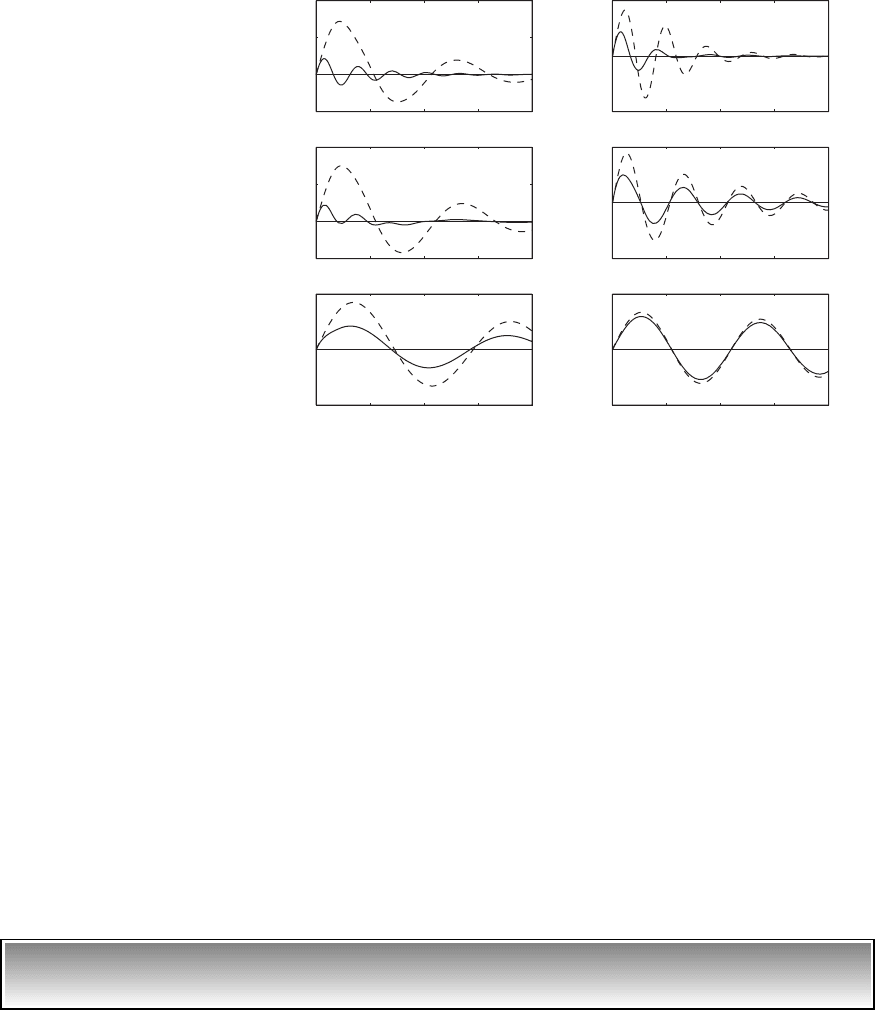
mass m

and broken lines are used to depict the response of the mass m

. As

expected, the free oscillations of the two masses show characteristics of

damped oscillations, and the long-time responses of these two masses settle

down to the equilibrium position; that is,

(8.88)

For m

 0.1, it is seen that the periods of the damped oscillations of the two

masses are different. As the mass ratio m

increases—that is, the mass m

in-

creases in comparison to the mass m

—the periods of damped oscillations of

both masses approach each other. As seen for single degree-of-freedom sys-

tems, the responses to initial velocity seen in Figure 8.11 and the responses to

impulses seen in Figure 8.9 have similar characteristics.

EXAMPLE 8.10

Damped free oscillations of a spring-mass system revisited

We return to Example 8.2 and solve for the free-oscillation response of a two

degree-of-freedom system by using Laplace transforms. The mass, stiffness,

and damping matrices used in Examples 7.20 and 8.9 are used to generate the

numerical results for the following initial conditions:

lim

t씮 q

1t 2 0

and

lim

t씮 q

1t 2 0

478 CHAPTER 8 Multiple Degree-of-Freedom Systems

0 10 20 30 40





0.1

0 10 20 30 40



()/(V

/

)

()/(V

/

)



0 10 20 30 40

5





0 10 20 30 40





0.1

0 10 20 30 40





0 10 20 30





(a) (b)

FIGURE 8.11

Responses of m

and m

when the masses are each subjected to the same initial velocity for

different mass ratios m

, z

 0.1, z

 0.2, and different values of v

: (a) v

 0.3 and

(b) v

 0.865. [Solid line x

(t); dashed line x

(t).]

(a)

In Eqs. (a) of Example 8.2, d  0.1.

For the initial conditions given in Eqs. (a), Eqs. (8.81) reduce to

(b)

From Eqs. (a) of Example 7.20 and Eqs. (7.41), we determine the following

quantities:

(c)

Furthermore, for the constant modal damping case of Example 8.9, we found

that

(d)

By using Eqs. (8.61), we determine that

(e)

Upon substituting the values given in Eqs. (c), (d), and (e) into

Eqs. (8.64), (8.67) and (b), we obtain

(f)K

1s 20.1s  0.0147

1s 2 0.1s  0.0238

1s 2 s

 0.282s

 4.573s

 0.479s  2.889

E1s2 s

 0.115s  1.556

C1s2 0.032s  0.889

B1s2 0.071s  2

A1s2 s

 0.167s  3



0.654

0.246

 2.662



0.246

2  2.7  2.722

 0.017



0.332

2  1.2  2.887

 0.048

 0.654 N

s/m

 0.246 N

s/m

 0.332 N

s/m

 0.943,

 2.25,

and



 0.75

 2.887 rad/s,

 2.722 rad/s

d5s  2z

12  c

1s 23s  2z

11  c

24d  2z

 d5s  2z

 4z

1s 2 3s  2z

 2z

4d  2z

10 2 d m,

10 2 0 m/s,

10 2d m,

and

10 2 0 m/s

8.4 Laplace Transform Approach 479