Baumgarte T., Shapiro S. Numerical Relativity. Solving Einstein’s Equations on the Computer

Подождите немного. Документ загружается.

6.2 Finite difference methods 191

neighboring grid points. To do so we can write the function values at these neighboring

grid points in terms of a Taylor expansion about the grid point i, and then combine these

expressions in such a way that all terms up to a desired order cancel out. For centered,

second-order derivatives, we only need the immediate neighbors, i.e., the grid points i + 1

and i − 1, but for higher-order expressions a larger number of grid points is required. As

an example, we ask the reader to work out the ﬁrst and second derivative of a function to

fourth order in the exercise below.

Exercise 6.6 Show that centered, fourth-order ﬁnite difference representations of

the ﬁrst and second derivatives of a function f are given by

(∂

f )

12x

( f

i−2

− 8 f

i−1

+ 8 f

i+1

− f

i+2

) (6.23)

and

(∂

f )

12(x)

(− f

i−2

+ 16 f

i−1

− 30 f

+ 16 f

i+1

− f

i+2

), (6.24)

where we have omitted the truncation error,

O(x

6.2.2 Elliptic equations

As an example of a simple, one-dimensional elliptic equation consider

∂

f = s. (6.25)

For concreteness, let us assume that the solution f is a symmetric function about x = 0,

in which case we can restrict the analysis to positive x and impose a Neuman condition at

the origin,

∂

f = 0atx = 0. (6.26)

(Note that antisymmetry would result in the Dirichlet condition f = 0atx = 0.) Let us

also assume that f falls off with 1/x for large x, which results in the Robin boundary

condition

∂

(xf) = 0asx →∞. (6.27)

We will further assume that the source term s is some known function of x.

We now want to solve the differential equation (6.25) subject to the boundary conditions

(6.26) and (6.27) numerically. To do so, we ﬁrst have to construct a numerical grid that

covers an interval between x

min

= 0andx

max

. Unless we compactify

the physical interval

[0, ∞] with the help of a new coordinate, for example ξ = x/(1 + x), ﬁnite computer

To compactify is to bring the outer boundary at x =∞into a ﬁnite value ξ<∞ by means of a coordinate transfor-

mation from x to ξ .

192 Chapter 6 Numerical methods

x = 0 x = x

gridpoints gridcells

i = 0 1 2 3 4 5 6 7 8 9

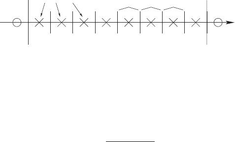
Figure 6.2 A cell-centered grid with eight grid points. The virtual grid points 0 and 9 lie outside of the domain

between x = 0andx = x

max

and do not need to be allocated in the computational grid.

resources will allow a uniform grid to extend to only a ﬁnite value x

max

. We then divide

the interval [x

min

, x

max

] into N grid cells, leading to a grid spacing of

x =

max

− x

min

. (6.28)

We can choose our grid points to be located either at the center of these cells, which would

be referred to as a cell-centered grid, or on the vertices, which would be refered to as a

vertex-centered grid. For a cell-centered grid we have N grid points located at

= x

min

+ (i − 1/2)x, i = 1,...,N, (6.29)

whereas for a vertex centered grid we have N + 1 grid points located at

= x

min

+ (i − 1)x, i = 1,...,N + 1. (6.30)

For now, the difference between between cell-centered and vertex-centered grids only

affects the implementation of boundary conditions, but not the ﬁnite difference represen-

tation of the differential equation itself. For concreteness, we will use a cell-centered grid

as illustrated in Figure 6.2.

We are now ready to ﬁnite difference the differential equation (6.25) together with the

boundary conditions (6.26) and (6.27). We deﬁne two arrays, f

and s

, which represent

the functions f and s at the grid points x

for i = 1,...,N .

In the interior of our domain

we can represent the differential equation (6.25)as

i+1

− 2 f

+ f

i−1

= (x)

i = 2,...,N − 1, (6.31)

where we have used the second-order expression (6.22) for the second derivative of f .

At the lower boundary point i = 1 the neighbor i − 1 does not exist in our domain, and,

similarly, at the upper boundary point i = N the point i + 1 does not exist. At these points

we have to implement the boundary conditions (6.26) and (6.27), which can be done in

many different ways.

One approach is the following. Consider, at the lower boundary, the virtual grid point

, positioned at x =−x/2. The two grid points x

and x

then bracket the boundary

point x

min

= 0 symmetrically. Using the centered differencing (6.21) we can then write the

In many computing languages, including C++, the ﬁrst element of an array is refered to as i = 0.

6.2 Finite difference methods 193

boundary condition (6.26)as

(∂

f )

1/2

− f

x

= 0, (6.32)

= f

, (6.33)

to second order in x.Fori = 1 we can now insert equation (6.33) into equation (6.31),

which yields

i+1

− f

= (x)

i = 1. (6.34)

We have used the virtual grid point x

to formulate the lower boundary condition, but it

does not appear in the ﬁnal ﬁnite difference equation, and therefore does not need to be

included in the computational arrays.

We can use a similar strategy at the upper boundary. With the help of a virtual grid point

N +1

we can write the boundary condition (6.27) to second order in x as

N +1

+ x

. (6.35)

We can again insert this into (6.31)fori = N and ﬁnd



+ x

− 2



+ f

i−1

= (x)

i = N . (6.36)

Equations (6.31), (6.34) and (6.36) now form a coupled set of N linear equations for

the N elements f

that we can write as







−110000 0

1 −21 0 0 0 0

00 0

001−21 0 0

000

00001−21

000001x

/(x

+ x) − 2













N −1







= (x)







N −1







(6.37)

or, in a more compact form,

A · f = (x)

S. (6.38)

The solution is given by

f = (x)

−1

· S, (6.39)

where A

−1

is the inverse of the matrix A, so that we have reduced the problem to inverting

an N × N matrix. All equations entering (6.37) are accurate to second order, so that

194 Chapter 6 Numerical methods

the solution f approaches the correct solution with (x)

as the leading order error

term.

The matrix A is tridiagonal, meaning that the only nonzero entries appear on the

diagonal and its immediate neighbors. This helps tremendously, since tridiagonal matrices

can be inverted quite easily at small computational cost,

even for moderately large N .

In particular, matrix inversion of tridiagonal matrices can be implemented in a way that

does not require storing all N

elements (the vast majority of which vanish anyway), but

instead only the diagonal band with its two neighbors.

The situation becomes more complicated in higher dimensions. Consider, for example,

Poisson’s equation in Cartesian coordinates in ﬂat space,

∇

f = ∂

f + ∂

f = s. (6.40)

We now construct a 2-dimensional grid in complete analogy to the 1-dimensional grid

discussed above. We will denote the N

grid points along the x-axis by x

, and the N

grid

points along the y-axis by y

. The functions f (x, y)ands(x, y) are then represented on a

2-dimenional grid and we write, for example,

i, j

= f (x

, y

). (6.41)

If we choose equal grid spacing in the x and y directions,  = x = y, we can ﬁnite

difference equation (6.40)as

i+1, j

+ f

i−1, j

+ f

i, j+i

+ f

i, j−1

− 4 f

i, j

= 

i, j

. (6.42)

As before we can write these coupled, linear equations (together with ﬁnite difference

representations of the boundary conditions) as one big matrix equation provided we absorb

the 2-dimensional arrays f

i, j

and s

i, j

into 1-dimensional vector arrays. We can do this, for

example, by constructing vector arrays F

and S

of length N

× N

, where the super-index

I ,givenby

I = i + N

( j − 1), (6.43)

runs over the entire 2-dimensional grid (i, j ) (see Figure 6.3). Given a super-index I we

can reconstruct i and j from

j = I mod N

+ 1 (6.44)

i = I − N

( j − 1). (6.45)

Exercise 6.7 Consider a 3-dimensional grid of size N

× N

. Construct a 1-

dimensional index I that runs over the entire grid (i, j, k), and provide expressions

that recover i, j and k from I.

See, e.g., Press et al. (2007).

6.2 Finite difference methods 195

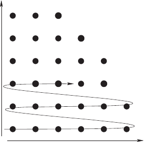
Figure 6.3 An illustration for a super-index I that sweeps through a 2-dimensional grid (i, j).

We can now write (6.42)as

I +1

+ F

I −1

+ F

I +N

+ F

I −N

− 4F

= 

(6.46)

and cast the problem as a matrix equation for the vector F

. For grid points (i, j)inthe

interior (i.e., away from the boundaries) the equation takes the form







··· 1 ··· 1 −41··· 1 ···













I −N

I −1

I +1

I +N







= 







I −N

I −1

I +1

I +N







. (6.47)

Evidently the matrix A is no longer tridiagonal. If the boundary conditions cooperate (and

they often do), it still is band diagonal, however, which means that the only nonvanishing

elements reside on bands parallel to the diagonal (this is also called “tridiagonal with

fringes”). The size of A is now N

× N

, but special software exists that takes

advantage of the band-diagonal structure, and requires storing only those nonvanishing

bands. In this case we need ﬁve bands. Exercise 6.7 shows that even for a 2-dimensional

covariant Laplace operator, as opposed to the ﬂat Laplace operator in equation (6.40), we

are already up to nine nonvanishing bands.

196 Chapter 6 Numerical methods

Exercise 6.8 Instead of Poisson’s equation in ﬂat space as given by equation (6.40),

consider the 2-dimensional covariant version,

∇

f =∇

∇

f = g

∇

f = g

∂

f − 

∂

f = s. (6.48)

Here the indices a and b only run over x and y, f is a scalar function, and 



. Do not assume the metric g

to be diagonal. Retrace the steps that led from

the differential equation (6.40) to the ﬁnite difference matrix equation (6.47)and

ﬁnd the matrix A (away from the boundaries).

Not surprisingly, the problem becomes even more involved in three dimensions. Exercise

6.9 shows that a covariant Laplace operator in three dimensions leads to 19 nonvanishing

bands in matrix A.

Exercise 6.9 Consider Poisson’s equation in three spatial dimensions in ﬂat space,

∂

f + ∂

f = s. (6.49)

(a) Retracing the steps from equation (6.40) to equation (6.47), determine the struc-

ture of the matrix A.

(b) Consider the covariant Laplace equation (6.48) in three dimensions and Cartesian

coordinates and ﬁnd A for this problem.

The problem becomes so large, especially in three dimensions, that solving the equa-

tions by direct matrix inversion is either impossible or impractical; it simply becomes

too expensive computationally. We therefore have to look for alternative methods of

solution.

Sticking with our example in two dimensions, another approach becomes apparent if

we rewrite equation (6.42)intheform

i, j

( f

i+1, j

+ f

i−1, j

+ f

i, j+i

+ f

i, j−1

) −



i, j

. (6.50)

Evidently, ﬁnite differencing the ﬂat-space Laplace operator results in each grid function

at every grid point being directly related to the average value of its nearest neighbors. We

could then start with an initial guess for a solution and then sweep through the grid and

update f

i, j

at each grid point according to equation (6.50). This approach is an exam-

pleofarelaxation scheme. Many variations are possible. If we only use values from

the previous sweep on the right hand side of equation (6.50), this scheme is known as

Jacobi’s method; if instead we use values that have already been updated in the cur-

rent sweep, it is called the Gauss–Seidel method, which converges faster. Unfortunately,

neither method converges rapidly enough to be of much practical use, even on modest

grids.

An improvement over these methods is most easily explained in terms of the residual

i, j

at each grid point, deﬁned as

i, j

= f

i+1, j

+ f

i−1, j

+ f

i, j+i

+ f

i, j−1

− 4 f

i, j

− 

i, j

, (6.51)

6.2 Finite difference methods 197

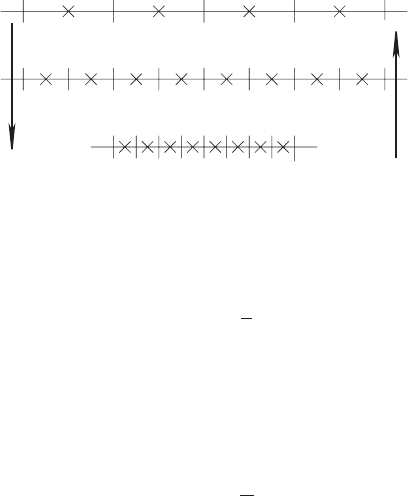
Prolongation Restriction

Figure 6.4 An illustration of a multigrid method.

which measures the deviation between the right-hand and left-hand sides of equation (6.42).

In terms of the residual we can write Jacobi’s method as

N +1

i, j

= f

i, j

, (6.52)

where the superscript N labels the N th sweep through the grid. This recipe implies that

in each sweep we correct each grid point by adding a number that is proportional to the

local residual. The idea behind successive overrelaxation (SOR) is to overcorrect each grid

point, and to modify equation (6.52) according to

N +1

i, j

= f

i, j

, (6.53)

where ω is some positive number. We refer to ω<1 as underrelaxation, and to 1 <ω<2

as overrelaxation; for values of ω larger than two the scheme does not converge. For a

good choice of ω, with 1 <ω<2, overrelaxation can improve convergence signiﬁcantly.

For most applications in three dimensions even SOR is not sufﬁciently fast, so that

alternative techniques are needed. One alternative is a multigrid method, which combines

the advantages of direct solvers and relaxation.

In multigrid methods, which we illustrate in Figure 6.4, the numerical solution is com-

puted on a hierarchy of computational grids with increasing grid resolution. The ﬁner

grids may or may not cover all the physical space that is covered by the coarser grids. The

numerical solution is then computed by completing sweeps through the grid hierarchy.

The coarse grid is sufﬁciently small so that we can compute a solution with a direct solver

(i.e., direct matrix inversion). This provides the “global” features of the solution, albeit

on a coarse grid and hence with a large local truncation error. We then interpolate this

approximate solution to the next ﬁner grid. This interpolation from a coarser grid to a ﬁner

grid is called a “prolongation”, and we point out that the details of this interpolation depend

on whether the grid is cell-centered (as illustrated in Figure 6.4) or vertex-centered. On

the ﬁner grid we can then apply a relaxation method, for example a Gauss–Seidel sweep.

While this method is too slow to solve the problem globally, as we have discussed above,

it is very well suited to improve the solution locally. This step is often called a “smoothing

An introduction to multigrid and “full approximation storage” methods, together with references, can be found in

Press et al. (2007).

198 Chapter 6 Numerical methods

sweep”. After this smoothing sweep the solution can be prolonged to the next ﬁner grid,

where the procedure is repeated. Once we have smoothed the solution on the ﬁnest grid, we

start ascending back to coarser grids. The interpolation from a ﬁner grid to a coarser grid

is called a “restriction”. The coarser grids now “learn” from the ﬁner grids by comparing

their last solution with the one that comes back from a ﬁner grid. This comparison provides

an estimate for the local truncation error, which can be accounted for with the help of an

artiﬁcial source term. On each grid we again perform smoothing sweeps, again improving

the solution because we inherit the smaller truncation error from the ﬁner grids. On the

coarsest grid we again perform a direct solve, as on the ﬁner grids with an artiﬁcial source

term that corrects for the truncation error, to improve the global features of the solution.

These sweeps through the grid hierarchy can be repeated until the solution has converged

to a predetermined accuracy.

Another popular method is the conjugate gradient method, which is also designed

for large, sparse matricies. There are discussions in the literature where the method is

implemented for applications in numerical relativity.

The good news is that several software packages that provide many of the most efﬁcient

and robust elliptic solvers are publically available. These routines are all coded up, including

for parallel environments.

With the help of these packages the user “only” needs to specify

the elements of the matrix A (preferably in some band-diagonal structure so that only the

nonvanishing bands need to be stored) together with the source term s on the right hand

side. The user can then choose between a number of different methods to solve the elliptic

equations.

Before closing this section we brieﬂy discuss nonlinear elliptic equations. Consider an

equation of the form

∇

f = f

g, (6.54)

where g is a given function and n is some number. Equation (6.54) reduces to the linear

equation (6.40) when n = 0. The equation is still linear for n = 1 and, upon ﬁnite differ-

encing, again gives rise to coupled, linear equations that are straighforward to solve by the

same matrix techniques discussed above. We note that equation (4.9) for the lapse function

α in maximal slicing contains a linear source term of this form, with n = 1. But what about

the situation for other values of n, resulting in a nonlinear equation for f ? For example,

the Hamiltonian constraint (3.37) for the conformal factor ψ contains several source terms

with n = 1, n = 5andn =−7.

As we shall now sketch, we can solve such a nonlinear

See, e.g., Oohara et al. (1997).

Examples include PETSc, available at acts.nersc.gov/petsc/,andLAPACK, available at

www.netlib.org/lapack/. Some of the algorithms discussed above are also implemented as modules

(or “thorns”) within Cactus (available at www.cactuscode.org), a parallel interface for performing large-scale

computations on multiple platforms.

We remind the reader that, depending on the sign of the exponent n, the solution to equation (6.54) may not be unique;

see exercise 3.8 for an example.

6.2 Finite difference methods 199

equation with very similar matrix techniques, provided we linearize the equation ﬁrst and

then iterate to get the nonlinear solution.

Let us denote the solution after N iteration steps as f

. We could take a very crude

approach and insert f

on the right-hand side of equation (6.54) and solve for the next

iteration f

N +1

on the left-hand side. Deﬁning the correction δ f from

N +1

= f

+ δ f (6.55)

we can write this scheme as

∇

δ f =−∇

+ ( f

)

g. (6.56)

The right-hand side is the negative residual of the equation after N steps,

=∇

− ( f

)

g, (6.57)

so equation (6.56) becomes

∇

δ f =−R

(not recommended). (6.58)

Evidently this is now a linear equation for the corrections δ f , which we can solve with the

methods discussed above. The corrections δ f also become smaller as the residual decreases,

as one would hope. We can do much better, however, and construct an iteration that

converges much faster, by inserting equation (6.55) on the right-hand side of equation (6.54)

as well and using a Taylor expansion

( f

N +1

)

= ( f

)

+ n( f

)

n−1

δ f + O(δ f

). (6.59)

We truncate after the linear term (so that the resulting equation is still linear), insert into

(6.54), and ﬁnd

∇

δ f − ng( f

)

n−1

δ f =−R

(recommended). (6.60)

We can think of the difference between equation (6.58) and equation (6.60)ashaving

truncated the Taylor expansion after the ﬁrst term on the right-hand side of equation (6.59),

and thereby retaining only the ﬁrst term on the left-hand side in equation (6.60). Clearly

we expect faster convergence for the latter, which usually is the case.

The price that we pay for the faster convergence is the new term involving δ f that

appears on the left-hand side of (6.60). The good news is that this term can be dealt with

quite easily. Equation (6.60)isoftheform

∇

f + uf = s, (6.61)

where, comparing with the model equation (6.25) that we considered above, the term uf

is new. The exact ﬁnite difference form of this equations depends on what kind of Laplace

operator we are dealing with. For a ﬂat Laplace operator in two dimensions, for example,

we could ﬁnite difference (6.61)as

i+1, j

+ f

i−1, j

+ f

i, j+i

+ f

i, j−1

+ (u

i, j

− 4) f

i, j

= 

i, j

. (6.62)

200 Chapter 6 Numerical methods

n+1

j j+1

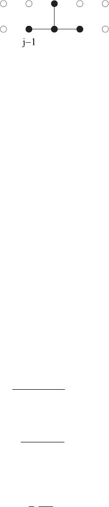
Figure 6.5 The ﬁnite-differencing stencil for the “forward-time centered-space” (FTCS) differencing scheme.

Comparing with (6.42) we see that the new term uf only affects the coefﬁcient of the

element f

i, j

. In the resulting matrix equation (6.47) we can therefore account for this

new term by adding u

i, j

to the diagonal of the matrix A. To solve equation (6.60), we

simply subtract ng( f

)

n−1

from the diagonal. This can be done very easily, and leads to a

signiﬁcantly faster iteration than using equation (6.58).

6.2.3 Hyperbolic equations

We now turn to hyperbolic equations. As a model of hyperbolic equations, consider a

“scalar” version of equation (6.7)

∂

u + v∂

u = 0. (6.63)

Equation (6.63) is sometimes referred to as the model advective equation, for obvious

reasons. For simplicity it does not contain any source terms, and the wave speed v is

constant. The equation is satisﬁed exactly by any function of the form u(t, x) = u(x − vt).

In contrast to the elliptic equations of Section 6.2.2 the equation has a time derivative in

addition to the space derivative, and thus requires initial data. A ﬁnite difference represen-

tation of this time derivative must involve at least two neighboring time levels. We will

ﬁrst consider two-level schemes.

As we have seen in Section 6.2.1, we can achieve a second-order differencing scheme

for the space derivative in equation (6.63) by using the centered ﬁnite difference expression

(∂

j+1

− u

j−1

2x

O(x

). (6.64)

Since we have decided to use a two-level scheme, a one-sided and ﬁrst-order expression

(∂

n+1

− u

t

O(t) (6.65)

for the time derivative will have to sufﬁce for now. Inserting both ﬁnite-difference repre-

sentations into equation (6.63) we can solve for u

n+1

and ﬁnd

n+1

= u

−

t

x

j+1

− u

j−1

). (6.66)

For reasons that are quite obvious this differencing scheme is called forward-time centered-

space, or FTCS (see Figure 6.5). It is an example of an explicit scheme, meaning that we