Baumgarte T., Shapiro S. Numerical Relativity. Solving Einstein’s Equations on the Computer

Подождите немного. Документ загружается.

6.2 Finite difference methods 211

two time levels, and, as in our discussion in Section 6.2.3, such averaging leads to the

Crank–Nicholson scheme

n+1

= φ

κt

2(x)



(φ

n+1

j+1

− 2φ

n+1

+ φ

n+1

j−1

) + (φ

j+1

− 2φ

+ φ

j−1

)



. (6.97)

This scheme is second order in both space and time, and exercise 6.19 showsthatitis

unconditionally stable.

Exercise 6.19 Perform a von Neumann stability analysis for the Crank–Nicholson

scheme (6.97), ﬁnd the ampliﬁcation factor and show that the scheme is uncondi-

tionally stable.

We close this section by recalling that wave equations can be written as the coupled

system (6.5), where, similar to the parabolic equation (6.90), the second equation contains

a ﬁrst time derivative and a second space derivative (but of opposite sign). Not surprisingly,

the computational methods discussed in this section are useful for integrating (hyperbolic)

wave equations as well. Since the 3 + 1 equations and other decompositions related to

it are quite similar to equation (6.5) in structure, these methods are important for many

applications in numerical relativity.

6.2.5 M esh reﬁnement

As we have discussed in Section 6.2.1, many current numerical relativity codes use a

uniform grid spacing to cover the entire spatial domain. Given that computational resources

are limited, so that we can afford only a ﬁnite number of grid points, such a “unigrid”

implementation may pose a problem, especially for a dynamical simulation in three spatial

dimensions. Imagine, for concreteness, a simulation of a strong-ﬁeld gravitational wave

source, like a compact binary containing neutron stars or black holes. On the one hand

we have to resolve these sources well, so as to minimize truncation error in the strong-

ﬁeld region. On the other hand, the grid must extend into the weak-ﬁeld region at large

distances from the sources, so as to minimize error from the outer boundaries and to

enable us to extract the emitted gravitational radiation accurately (see Chapter 9). One

possible solution to this classic “dynamic range” problem is to introduce a new coordinate

system that serves to cover a larger spatial region for the same number of grid points.

For example, replacing a uniform radial grid by one proportional to the logarithm of the

radius can extend the computational domain out to larger distances for the same number

of grid points. It is also possible to introduce a coordinate system that maps spatial inﬁnity

to a ﬁnite coordinate value (“compactiﬁcation”).

These approaches, however, may also

introduce new problems. Consider, for example, the propagation of outgoing gravitational

radiation. Its physical wavelength is ﬁxed but in these new coordinate systems that have

Recall the discussion following equation (6.27), which suggests why compactiﬁcation can be particularly useful for

imposing asymptotic boundary conditions.

212 Chapter 6 Numerical methods

their highest spatial resolution in the strong-ﬁeld near zone the radiation is resolved by

fewer and fewer grid points as it propagates out to larger distances. This effect may thus

spoil the quality of wave extraction if the coordinate transformations are too naive.

Exercise 6.20 Show how radial resolution diminishes with increasing radius r for

a grid that is uniform in the logarithmic coordinate y = ln r.

A very promising alternative is mesh reﬁnement, which has been widely developed

and used in the computational ﬂuid dynamics community and is becoming increasingly

popular in numerical relativity. In fact, adaptive mesh reﬁnement was instrumental in the

discovery of critical phenomena in general relativity

and has played a key role in the

simulations of binary black holes.

The basic idea underlying mesh reﬁnement techniques is to perform the simulation not

on one numerical grid, but on several, as in the multigrid methods for elliptic equations that

we discussed in Section 6.2.2 (see Figure 6.4). A coarse grid covers the entire space, and

extends to large physical separations. Wherever ﬁner resolution is needed to resolve small-

scale structures, as is the case, for example, of a compact binary emitting gravitational

radiation, a ﬁner grid is introduced. Typically, the grid spacing on the ﬁner grid is half that

on the next coarser grid, but clearly other reﬁnement factors can be chosen. The hierarchy

can be extended, and typical mesh reﬁnement applications employ multiple reﬁnement

levels.

While the concept is quite simple, many of the details and the implementation of mesh

reﬁnement are fairly subtle. In particular, the boundary conditions imposed on the reﬁned

grids have to be posed and implemented with some care, since otherwise waves will reﬂect

off these interfaces, leading to spurious numerical artifacts.

Two versions of mesh reﬁnement can be implemented. In the simpler version, called

ﬁxed mesh reﬁnement or FMR, it is assumed that the reﬁned grids will be needed only

at known locations in space that remain ﬁxed throughout the simulation. The center of

a pulsating star, for example, may remain ﬁxed at the origin, so that nested reﬁnements

boxes of ﬁxed size and centered at the origin are adequate to reﬁne the computational

domain. The situation is more complicated for objects that are moving, as is the case for a

coalescing binary star system. In this case we do not know a priori the trajectories of the

companion stars, hence do not know which regions need reﬁning. Moreover, these regions

will be changing as the system evolves and the stars move. Clearly, we would like to move

the reﬁned grids with the stars. Such an approach, whereby the grid is relocated during the

simulation to give optimal resolution at each time step, is called adaptive mesh reﬁnement

or AMR.

An example of an AMR implementation in numerical relativity, simulating the

See Chapter 8.4.

See Chapter 13.

A discussion of these issues in the context of numerical relativity can be found, for example, in Schnetter et al. (2004)

and the references therein.

See Berger and Oliger (1984).

6.3 Spectral methods 213

Figure 6.10 A simulation of neutron star coalescence using adaptive mesh reﬁnement. Shown are the lapse

function at an early time before merger (left panel) and a late time after merger (right panel) in the inner part of

the computational grid, together with a mesh (representing every other grid point used in the simulation) that

shows how the reﬁnement levels track the motion of the neutron stars. [From Evans et al. (2005).]

head-on collision of two neutron stars, is shown in Figure 6.10. Other examples utilizing

FMR and AMR will be cited when we discuss applications in later chapters.

6.3 Spectral methods

A general introduction to spectral methods can be found in several books and monographs

on the subject.

Applications to numerical relativity have been described in many papers

and review articles.

Here we shall restrict our own discussion to a brief summary of some

of the key features of spectral methods.

6.3.1 Representation of functions and derivatives

Spectral methods approximate the solution to a differential equation, say u(x), as a truncated

series in some complete set of basis functions φ

(x),

u(x)  u

(N )

(x) =



k=0

(x). (6.98)

Here the coefﬁcients

, which do not depend on x, are called the spectral coefﬁcients.

Evidently we can express derivatives of u

(N )

(x) analytically in terms of derivatives of the

known basis functions φ

(x), for example

∂

(N )

(x) =



k=0

∂

(x). (6.99)

See, e.g., Gottlieb and Orszag (1977)andBoyd (2001).

See, e.g., Bonazzola et al. (1999b), Gourgoulhon (2002)andPfeiffer et al. (2003b). Our treatment draws signiﬁcantly

from the discussions in these references.

214 Chapter 6 Numerical methods

Given that we can represent derivative operators exactly, and given that for many applica-

tions contributions from the higher order basis functions φ

decrease very quickly with k,

the numerical error in spectral methods often drops off exponentially with N . To achieve

the same accuracy as ﬁnite difference methods (for which the error typically falls of with

some small power of the number of gridpoints N ), spectral methods often require signif-

icantly fewer computational resources, which makes them a very powerful and attractive

alternative. On the downside, spectral methods are often more complicated to implement

then ﬁnite difference methods, and they are less suitable for the modeling of situations in

which discontinuities (in either functions or their derivatives) may occur.

The general idea underlying spetral methods is to write all expressions in the differ-

ential equation and its boundary conditions in terms of the N + 1 basis functions φ

(x).

We then derive and solve a set of N + 1 equations for the N + 1 spectral coefﬁcients.

The approximate solution u

(N )

(x) is then given in terms of the spectral coefﬁcients by

equation (6.98). Several choices have to be made along the way – in particular we have

to pick a set of basis functions, and we have to decide how exactly to construct the

conditions on the spectral coefﬁcients imposed by the differential equation – but before

discussing these in more general terms it may be useful to work through a simple example

problem.

6.3.2 A simple example

Consider the 1-dimensional, linear differential equation

∂

u − (x

+ 3x

)u = 0, (6.100)

subject to the boundary conditions

u(−1) = u(1) = 1. (6.101)

The exact solution to this equation is given by

u(x) = exp



− 1



. (6.102)

For basis functions φ

(x) we could simply use polynomials x

, but to satisfy the boundary

conditions (6.101) automatically we will instead employ a polynomial expansion in the

form

(N )

= 1 + (1 − x

)(

x +

+···+

). (6.103)

This section follows Section 1.2 of Boyd (2001), who provides this example.

This expansion is not exactly in the form of equation (6.98), but nevertheless illustrates very nicely some of the

important properties of spectral solutions.

6.3 Spectral methods 215

Our goal now is to determine the coefﬁcients

in such a way so as to make the residual,

deﬁned as

(N )

= ∂

(N )

− (x

+ 3x

(N )

, (6.104)

small. It is not clear, a priori, how to measure the size of this residual. One possible

approach is to evaluate the residual at several points x

For concreteness, assume N = 2, in which case the residual (6.104) becomes

(2)

= (2

+ 2

) − 6

x − (3 + 3

+ 12

− 3

+3(

−

+ 3

+ (−1 −

+ 3

(6.105)

−

+ (

−

+ 10

We now need three equations for the three unknown coefﬁcients

and

,sowe

evaluate this residual at three points, say x

=−1/2, x

= 0, and x

= 1/2. The resulting

set of linear equations can be represented as the matrix equation







659

256

−

1683

512

1171

1024

−20 2

659

256

−

1683

512

1171

1024

























−







. (6.106)

The solution is given by

=−

784

3807

= 0. (6.107)

Given the structure of the differential equation (6.100) and the boundary condition (6.101)

we could have guessed that the solution must be symmetric, which implies that all odd

coefﬁcients

, including

, must be zero. That means that we only had to search for two

coefﬁcients rather than three, illustrating the fact that it is often useful to think about the

solution before constructing it numerically. This also means that

must be zero as well,

so that our solution’s leading order error term is the fourth order term.

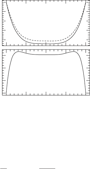
We plot our spectral solution, together with the exact solution and the error, in

Figure 6.11. The relative error is on the order of 2%, which is remarkable small given

that effectively we constructed the spectral solution with only two free parameters. Clearly,

it would not be possible to achieve this accuracy with only two grid points in a ﬁnite

difference approach. The accuracy of the spectral solution does depend, however, on the

choices that we have made along the way, namely the basis functions φ

and the evaluation

of the residual. In this simple example problem we have made more or less ad hoc choices,

partly motivated by the boundary conditions. In the next section we will discuss “smarter”

choices that are known to work well under quite general circumstances.

216 Chapter 6 Numerical methods

0.95

0.9

0.85

0.8

0.015

(2)

− u

u, u

(2)

0.01

0.005

−1

−0.5

0.5

Figure 6.11 The top panel shows the exact solution u(x) (solid line) and the spectral solution u

(2)

(x )(dashed

line) to the differential equation (6.100), subject to boundary conditions (6.101). The bottom panel shows the

absolute error u

(2)

(x ) −u(x).

Exercise 6.21 The Chebychev polynomials T

(x) satisfy the differential equation

(1 − x

)

1/2



(1 − x

)

1/2

(x)



=−n

(x) (6.108)

on the interval [−1, 1]. Solutions T

(x) exist only for certain values of the eigenvalue

n, which have to be determined together with the solution. Show that regular solutions

satisfy the boundary conditions



= n

, x = 1,



=−n

, x =−1.

(6.109)

Even if we didn’t know already that the solutions are in fact polynomials we might

try expanding them in terms of polynomials,

(x) 



k=0

. (6.110)

For simplicity truncate at N = 2sothatT

(x)  a

+ a

x + a

, and express the

differential equation (6.108) and boundary conditions (6.109) in terms of the coefﬁ-

cients a

, a

and a

. You need three equations for the three coefﬁcients; two follow

from the boundary conditions, and so only one more condition needs to be supplied

by the differential equation. To get this last condition you could evaluate the differ-

ential equation at one point, e.g., x = 0. Instead, leave x undetermined and impose

the differential equation for an arbitrary value x

. Form a set of linear equations

for the coefﬁcients a

, a

and a

and show that you can ﬁnd nontrivial solutions

only for the eigenvalues n = 0, 1 and 2. Also ﬁnd the corresponding eigenvectors,

from which you can construct the Chebychev polynomials. Your solutions should be

6.3 Spectral methods 217

independent of x

, indicating that they satisfy the differential equation (6.108)atall

points, which in turn means that your solutions are not just approximate solutions,

but in fact give the correct lowest-order Chebychev polynomials (see equation 6.115

below).

6.3.3 Pseudo-spectral methods with Chebychev polynomials

Consider a differential equation

Lu(x) = s(x), (6.111)

subject to a suitable set of boundary conditions, where L is some differential operator, and

s(x) a source function. Our goal is then to ﬁnd a set of spectral coefﬁcients

associated

with the N th order expansion u

(x)ofu(x) so that the residual

R = Lu

(N )

− s (6.112)

becomes small. Different spectral methods differ in how this residual is evaluated.

For example, we could project the residual back into the basis functions φ

(x)by

performing an overlap integral of equation (6.112) with each of the functions φ

(x). If

the basis functions φ

(x) all satisfy the boundary conditions, this approach is called a

Galerkin method. If on the other hand the φ

(x) do not satisfy the boundary conditions

individually and therefore have to be combined in such a way that the combination satisﬁes

the boundary conditions – which results in extra equations for the spectral coefﬁcients –

this method is called a tau method.

Alternatively we can evaluate the residual (6.112) at a certain set of N + 1 points x

called the collocation points,toderiveN + 1 equations for the N + 1 spectral coefﬁcients

This approach, which we used in the simple example presented in Section 6.3.2,

is called a pseudo-spectral or collocation method. It is also the most popular method in

numerical relativity, and we will therefore focus on this approach.

We still have to choose a set of basis functions. For periodic problems, a Fourier expan-

sion in sines and cosines is recommended, but for most applications in numerical relativity

the most suitable set of basis functions are Chebychev polynomials.

The properties of

the Chebychev polynomials also suggest a particular choice for the collocation points.

Chebychev polynomials are deﬁned on the interval [−1, 1] as

(cos θ) = cos(nθ ) (6.113)

We may later have to replace some of these equations to account for the boundary conditions.

Boyd (2001) offers the following “Moral Principle 1”:

1. When in doubt, use Chebychev polynomials unless the solution is spatially periodic, in which case ordinary Fourier

series is better.

2. Unless you’re sure another set of basis functions is better, use Chebychev polynomials.

3. Unless you’re really, really sure that another set of basis functions is better, use Chebychev polynomials.

218 Chapter 6 Numerical methods

and satisfy the singular Sturm–Liouville problem

(1 − x

)

1/2



(1 − x

)

1/2

(x)



=−n

(x). (6.114)

The ﬁrst few polynomials are

(x) = 1,

(x) = x,

(x) = 2x

− 1, (6.115)

(x) = 4x

− 3x,

(x) = 8x

− 8x

+ 1,

(cf.exercise6.21). Higher-order polynomials can be constructed from the recurrence

relation

n+1

= 2xT

(x) − T

n−1

(x), (6.116)

which holds for n ≥ 1. Chebychev polynomials form a complete set and are orthogonal in

the interval [−1, 1] with a weight w(x) = (1 − x

)

−1/2

, T

) ≡

2 − δ



−1

(x)T

(x)w(x)dx = δ

, (6.117)

wherewehavedeﬁned(T

, T

), the scalar product between T

and T

The polynomial T

(x)hasN zeros in [−1, 1] located at

= cos



π(k + 1/2)



, k = 0, 1,...,N − 1. (6.118)

Between these zeros, the Chebychev polynomials take maxima of value 1 or minima of

−1 at locations

= cos



πk



, k = 0, 1,...,N. (6.119)

At the endpoints at x =±1 they take values

(−1) = (−1)

, T

(1) = 1. (6.120)

The facts that the Chebychev polynomials oscillate between +1and−1, and that two

successive Chebychev polynomials assume their extrema at locations that are staggered,

means that the truncation error due to the neglect of terms of order higher than N is spread

more or less “evenly” over the interval [−1, 1]. This feature is one of the properties that

makes these polynomials so attractive for spectral methods.

Using the orthogonality of the Chebychev polynomials, we can invert equation (6.98)

for Chebychev polynomials and compute the coefﬁcients

from

= (u, T

) =

2 − δ



−1

(x)u(x)w(x)dx. (6.121)

6.3 Spectral methods 219

In reality, however, we cannot evaluate this integral exactly on a computer. A very accurate

method for computing this integral is either Gauss integration, in which case the collocation

points are the N + 1 zeros of T

N +1

(x) (given by equation 6.118), or Gauss–Lobatto

integration, for which the collocation points are the N + 1 extrema of T

(x) (given by

equation 6.119). The latter set includes the boundary at x =±1, while the former does

not.

In the case of Gauss–Lobatto integration, the integral (6.121) for the scalar product

between u(x)andT

(x) reduces to the discrete expression



k=0

), (6.122)

wherewehavedeﬁned



2, k = 0ork = N ,

1, k = 1,...,N − 1,

(6.123)

and where the collocation points X

are given by the extrema (6.119). The u

are the values

of the function u(x) at the collocation points,

= u

(N )

) =



k=0

). (6.124)

Evidently, with the help of (6.122) and (6.124) we can transform back and forth between

the u

’s or the

’s, meaning that we can represent the function u

(N )

by either of the two sets.

Realizing that the Chebychev polynomials are just cosines in disguise (see their deﬁnition

equation 6.113), we can perform these transformations very efﬁciently with the help of

fast Fourier transform (FFT) techniques, which is another reason for the popularity of

Chebychev polynomials.

Evaluated at the collocation points, the orthogonality relation (6.117) becomes the

discrete expression



k=0

) = δ

. (6.125)

Exercise 6.22 Verify equation (6.125) by using equations (6.122)and(6.124).

6.3.4 Elliptic equations

For simplicity, imagine we want to solve the same 1-dimensional elliptic equation

∂

f (x) = s(x) (6.126)

considered at the beginning of Section 6.2.2. We now write all expressions in this equation

in terms of Chebychev polynomials. Before we can do this, we may ﬁrst have to perform

a coordinate transformation, since the Chebychev polynomials exist only on the interval

220 Chapter 6 Numerical methods

[−1, 1], whereas in the physical problem of interest the coordinate x may span a completely

different interval. In the following we assume that a suitable coordinate transformation has

been performed, so that the new coordinate x indeed covers the interval [−1, 1]. We then

expand the function f (x)as

f (x) =



k=0

(x). (6.127)

As we have said in Section 6.3.1, the beauty of spectral methods lies in the fact that we can

express derivatives of functions analytically in terms of derivatives of the basis functions,

so in this case

∂

f (x) =



k=0



(x), (6.128)

where the prime denotes a derivative with respect to x. The goal is now to express derivatives

of the Chebychev polynomials in terms of Chebychev polynomials themselves. To do that

the identities proven in exercise 6.23 will be useful.

Exercise 6.23 Show that derivatives of Chebychev polynomials satisfy the relation



(x) = 2nT

n−1

(x) +

n − 2



n−2

(x), n > 2, (6.129)

as well as T



(x) = 4T

(x), T



(x) = T

and, evidently, T



(x) = 0. Also show that



(x) = 2n(T

n−1

(x) + T

n−3

(x) + T

n−5

(x) +···+T

(x)), n even,



(x) = 2n(T

n−1

(x) + T

n−3

(x) + T

n−5

(x) +···+T

(x)) + nT

(x), n odd.

(6.130)

Given that the derivatives T



(x) are functions like any other, we can expand them as



(x) =



l=0

(x) (6.131)

where, according to equation (6.121), the coefﬁcients D

are the projections of T



(x) into

(x)givenby

= (T

, T



). (6.132)

Inserting equation (6.130)forl ≥ 0andk ≥ 0weﬁnd







01030 5 ···

00408 0 ···

0006010···

00008 0 ···

0000010···

00000 0 ···







. (6.133)