Baumgarte T., Shapiro S. Numerical Relativity. Solving Einstein’s Equations on the Computer

Подождите немного. Документ загружается.

6.2 Finite difference methods 201

can solve for the grid function u

n+1

at the new time level n + 1 directly in terms of function

values on the old time level n. This is a very convenient feature, because, given all the

values at the time level n, we can simply loop through the entire grid at the new time level

n + 1 and update each grid point independently of all the other grid points; i.e., the u

n+1

are uncoupled.

Unfortunately, however, FTCS is fairly useless. To see this, we perform a von Neumann

stability analysis, which is basically a linear eigenmode analysis to test a time-dependent

numerical scheme for stability. For constant coefﬁcients, as in the case of our model

equation (6.63), we can write the solution u(t, x) to our continuum hyperbolic differential

equation as a superposition of eigenmodes e

i(ωt+kx)

.Herek is a spatial wave number,

ω = ω(k) the wave frequency, and, at the risk of stating the obvious, i =

√

−1(andnot

a grid index). We can determine the dispersion relation between ω and k by inserting the

modal decomposition back into the differential equation. A real ω, for which e

iωt

has a

magnitude of unity, yields sinusoidally oscillating modes, while the existence of a complex

piece in ω leads to exponentially growing or damping modes. In the case of exponential

growth, the magnitude of e

iωt

will exceed unity.

We can perform a similar spectral analysis of the ﬁnite difference equation. Write the

eigenmode for u

= ξ

ik( j x )

. (6.67)

Here the quantity ξ plays the role of e

iωt

andiscalledtheampliﬁcation factor: u

ξu

n−1

= ξ

n−2

... = ξ

. We can ﬁnd the dependence of ξ on wave number k by

inserting equation (6.67) into the ﬁnite difference form of the differential equation. For the

scheme to be stable, the magnitude ξ must be smaller or equal to unity for all k,

|ξ(k)|≤1 von Neumann stability criterion. (6.68)

To perform a von Neumann stability anaylsis of the FTCS scheme we substitute the

decomposition (6.67)into(6.66) and ﬁnd

ξ(k) = 1 − i

vt

x

sin kx. (6.69)

Equation (6.69) shows that the magnitude of ξ is greater than unity for all k, indicating

that this scheme is unstable.Infact,wehave|ξ | > 1 independently of our choice for x

and t, which makes this scheme unconditionally unstable. That is bad.

Exercise 6.10 Derive equation (6.69).

The good news is that there are several ways of ﬁxing this problem. For example, we

could replace the term u

on the right-hand side of equation (6.66) by the spatial average

202 Chapter 6 Numerical methods

Domain of determinacy

stab

n+1

Figure 6.6 The Courant condition for many explicit ﬁnite difference implementations of hyperbolic equations

requires the new grid point for u

n+1

to lie inside the domain of derterminacy of the ﬁnite difference stencil on the

previous time level n.

j+1

+ u

j−1

)/2, in which case equation (6.66) becomes

n+1

j+1

+ u

j−1

) −

t

x

j+1

− u

j−1

). (6.70)

This differencing scheme is called the Lax method.

Exercise 6.11 Show that a von Neumann analysis for the Lax method results in the

ampliﬁcation factor

ξ = cos kx − i

vt

x

sin kx. (6.71)

The von Neumann stability criterion (6.68) then implies that we must have

|v|t

x

≤ 1

(6.72)

for stability. This is known as the Courant–Friedrichs–Lewy condition, or Courant con-

dition for short, and it holds for many explicit ﬁnite difference schemes for hyperbolic

equations. We call the ratio between |v|t and x the Courant factor.

Recalling that v represents the speed of a characteristic, we may interpret the Courant

condition in terms of the domain of determinacy that we introduced in Section 6.1. Consider

the situation sketched in Figure 6.6. The Courant condition (6.72) states that the grid point

for u

n+1

at the new time level n + 1 has to reside inside the domain of determinacy

of the interval spanned by the ﬁnite difference stencil at the time level n. This makes

intuitive sense: if u

n+1

were outside this domain, its physical speciﬁcation would require

more information about the past than we are providing numerically, which may trigger an

instability.

As we have seen, the Lax scheme is stable as long as we have chosen t sufﬁciently small

so that it satisﬁes the Courant conditon (6.72). This makes the Lax scheme conditionally

stable.

It seems somewhat like a miracle that simply replacing a grid function by a local average

manages to change the numerical scheme from unconditionally unstable to conditionally

stable. This change can be interpreted in very physical terms, however. Adding and sub-

tracting u

on the right hand side of equation (6.70) allows us to rewrite the equation

6.2 Finite difference methods 203

n+1

= u

j+1

− 2u

+ u

j−1

) −

t

x

j+1

− u

j−1

), (6.73)

n+1

− u

t

=−v

j+1

− u

j−1

2x

(x)

2t

j+1

− 2u

+ u

j−1

(x)

. (6.74)

But equation (6.74) is a ﬁnite-difference representation of the differential equation

∂

u + v∂

u = D ∂

u, (6.75)

where the term on the right-hand side is essentially a diffusion term, with parameter

D = (x)

/(2t) serving as a constant coefﬁcient of diffusion. Such a term is identical

to the one appearing in the right-hand side of the equations of particle and radiative

diffusion and thermal conduction. It is also similar to the dissipation term arising from

shear viscosity in the Navier–Stokes equation (see, e.g., the terms proportional to η on the

right hand side of 5.71). Clearly, in the context of the model advective equation, this term

is purely numerical in nature and disappears, for a constant Courant factor |v|t/x,in

the limit x → 0. We call this effect numerical viscosity; it tends to stabilize numerical

schemes, but also introduces numerical errors in the form of anomalous diffusion and

dispersion.

In particular, a Courant stability analysis for the Lax scheme shows that for

stable evolution the magnitude of the ampliﬁcation factor is always less than unity unless

|v|t ≡ x (in which case |ξ |=1); this feature implies the amplitude of any wave will

decrease spuriously with time as it propagates. A related effect is anomalous dispersion,

an additional price we pay for stablity in the Lax scheme and many other ﬁnite difference

schemes for hyperbolic systems. When the Courant factor is not precisely unity, there are

phase errors that arise for modes of different wave numbers k. Anomalous dispersion is

most serious for high wave modes kx

∼

1, corresponding to small length scales λ

∼

x.

But we should not really expect to be able to probe features on any scale unless we are

prepared to resolve that scale with many grid points, in which case anomalous dispersion

is usually not a problem.

The explicit addition of a diffusive term to the ﬁnite-difference representation of a

hyperbolic equation can sometimes be exploited to great advantage. If the term is of

sufﬁciently high order (e.g., ∂

where n ≥ 4) then such a term serves to damp the very

high frequency modes that can destabilize the numerical integration of an evolved variable.

Moreover, if such a dissipative term is explicilty multiplied by an overall factor (i.e.,

“diffusion coefﬁcient”) that is sufﬁciently small in magnitude, then the new term will

not otherwise distort the numerical solution appreciably. This is the basic idea behind the

implementation of Kreiss–Oliger dissipation

for stabilizing ﬁnite-difference integrations

The numerical viscosity introduced here should not be confused with the artiﬁcial viscosity introduced in Chapter 5.2.1.

Kreiss and Oliger (1973).

204 Chapter 6 Numerical methods

of hyperbolic systems. The technique has proven very useful for stabilizing many different

numerical integration schemes employed in numerical relativity.

There are a number of other ways of constructing stable ﬁnite-difference schemes

for the model equation (6.63). A popular alternative to the Lax scheme is upwind

differencing

n+1

− u

t

=−v











− u

j−1

x

,v>0

j+1

− u

x

,v>0.

(6.76)

This scheme borrows its name from the fact that for a wave with v>0, that travels “to the

right”, say, the new grid function u

n+1

is affected only by the “upwind” grid points to its

left, i.e., that lie in the region through which the wave travels before reaching x

Exercise 6.12 Consider the “left-sided” upwind scheme for v>0. Perform a von

Neumann stability analysis and show that this scheme is stable as long as the Courant

condition (6.72) is satisﬁed. Also show that the “left-sided” scheme is unstable for

v<0.

As written in equation (6.76) the upwind scheme treats even the spatial derivatives only

to ﬁrst order in x. This can be improved by replacing the right-hand sides with one-

sided, higher-order ﬁnite-difference approximations (for example with the stencil found in

exercise 6.5).

It would be desirable, however, to have a scheme that is second order in both space

and time. One way to construct such a code is to abandon two-level schemes, and instead

consider a three-level scheme. We can then construct centered derivatives both for the

time-derivative,

(∂

n+1

− u

n−1

2t

O(t

), (6.77)

and the space derivative (6.64). Putting these two together we have the leap-frog scheme,

n+1

= u

n−1

− v

t

x

n+1

− u

n−1

) (6.78)

(see Figure 6.7).

Exercise 6.13 Perform a von Neumann stability analysis to show that the leap-frog

scheme is stable, as long as the Courant condition (6.72) is satisﬁed, in which case

|ξ |=1 holds exactly. Thus demonstrate that there is no amplitude damping in this

scheme.

Some researchers prefer two-level schemes over three-level schemes because three-level

schemes require initial data on two different time levels, which can be somewhat awkward.

The leap-frog scheme has the additional disadvantage that, if picturing the computational

grid as a chess board, it only connects ﬁelds of the same color (see Figure 6.7). “Black”

6.2 Finite difference methods 205

n+1

j j+1

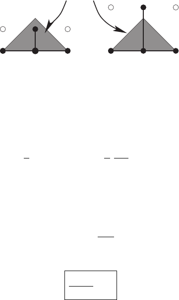
Figure 6.7 Finite difference stencil for the leap-frog scheme.

n+1

1 j j+1

Figure 6.8 Finite difference stencil for an implicit scheme.

grid points can therefore evolve completely independently of “white” grid points, and the

two sets of grid points may drift apart as numerical error accumulates differently for the

two sets of points. If necessary, this problem can be solved by artiﬁcially adding a very

small viscous term that links the two sets together. Once these potential issues are resolved,

leap-frog is a very simple, accurate and powerful method.

Yet another way of constructing a stable two-level scheme is to use backward time differ-

encing instead of forward differencing in evaluating the right-hand side of equation (6.66).

We simply evaluate the right-hand side of this equation at the time level n + 1 instead of

n (which results in a truncation error of the same linear order in t). This approach then

yields the “backward-time, centered-space” scheme,

n+1

= u

−

t

x

n+1

j+1

− u

n+1

j−1

) (6.79)

(see Figure 6.8). Performing a von Neumann stability analysis we ﬁnd the ampliﬁcation

factor

ξ =

1 + iC sin kx

, (6.80)

where C = vt/x is the Courant factor, and hence we obtain

|ξ(k)|≤1 (6.81)

for all values of t. This ﬁnding means that this scheme is unconditionally stable.The

size of the step size t is no longer restricted by stability, and instead is limited only by

accuracy requirements. As we will discuss in Section 6.2.4, this property is even more

206 Chapter 6 Numerical methods

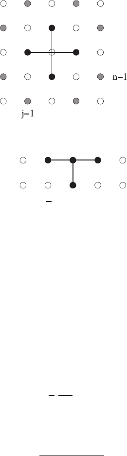
n+1

j j+1

Figure 6.9 Finite difference stencil for the Crank–Nicholson scheme.

important for parabolic equations, but we shall discuss some consequences already in the

present context.

The disadvantage of the backward differencing scheme (6.79) is that we can no longer

solve for the new grid function u

n+1

at the new time t

n+1

explicitly in terms of old

grid functions at t

alone. Instead, equation (6.79) now couples u

n+1

with the its closest

neighbors u

n+1

j+1

and u

n+1

j−1

. This coupling provides an implicit linear relation between the

new grid functions, and is therefore an example of an implicit ﬁnite-differencing scheme

(see Figure 6.8). We can no longer sweep through the grid and update one point at a time;

instead we now have to solve for all grid points simultaneously. Writing equation (6.79)

at all interior grid points, and then taking into account the boundary conditions, leads

to a system of equations quite similar to those we discussed in the context of elliptic

equations in Section 6.2.2. Inverting the resulting linear matrix equation directly may be

feasable in one spatial dimension (e.g., the matrix is tridiagonal in this example), but it

is much harder in higher dimensions. One way to approach this problem is to cast the

grid functions into a single vector array and call upon a routine designed to invert sparse

matricies. Another way is to deal with only one spatial dimension at a time, updating each

dimension in succession, and iterating until convergence. This later method is an example

of the alternating-direction implicit or ADI method.

The scheme (6.79) is still only ﬁrst order in time because we are using a one-sided

expression for the time derivative. A second-order scheme would be time-centered, meaning

that we should estimate the the time derivative at the mid-point between the two time levels

n and n + 1,

(∂

n+1/2

n+1

− u

t

O(t

). (6.82)

Implementing time-centering means that we also have to evaluate the space derivative at

this same midpoint n + 1/2, which we can do by averaging between the values at n and

n + 1. This approach yields the Crank–Nicholson scheme

n+1

= u

−

t

x



n+1

j+1

− u

n+1

j−1

) + (u

j+1

− u

j−1

)



, (6.83)

illustrated in Figure 6.9. Evidently, we can interpret the Crank–Nicholson scheme as the

average between the FTCS scheme (6.66) and the backwards differencing scheme (6.79).

Crank–Nicholson is second order in both space and time, and exercise 6.14 shows that it

is unconditionally stable.

6.2 Finite difference methods 207

Exercise 6.14 Perform a von Neumann stability analysis for the Crank–Nicholson

scheme (6.83)andshowthat

ξ =

1 + iβ

1 − iβ

, (6.84)

where β = (v/2)(t/x)sinkx,sothat|ξ (k)|=1 exactly.

As we found for the fully implicit method (6.79) it is not possible to solve for the new grid

functions u

n+1

in the Crank–Nicholson scheme (6.83) explicitly. An alternative to inverting

a tridiagonal matrix as in the implicit scheme described above (or the ADI approach in

multidimensions) is the iterative Crank–Nicholson scheme that uses a predictor-corrector

approach. In the predictor step we predict the new values u

n+1

by using the fully explicit

FTCS scheme (6.66)

(1)

n+1

= u

−

vt

2x

j+1

− u

j−1

), (6.85)

which, as we have seen above, would be unconditionally unstable by itself. In a subsequent

corrector step we use these predicted values

(1)

n+1

together with the u

to obtain a time-

centered approximation for the spatial derivative on the right hand side of equation (6.83).

This step yields the corrected values of the grid function,

(2)

n+1

= u

−

vt

4x



(

(1)

n+1

j+1

−

(1)

n+1

j−1

) + (u

j+1

− u

j−1

)



. (6.86)

The corrector step can be repeated an arbitrary number times N , always using the previous

values

(N −1)

n+1

on the right-hand side to ﬁnd new corrected values

(N )

n+1

. In principle

this iteration should converge to the Crank–Nicholson scheme (6.83), but the stability

analysis in exercise 6.15 shows that one must carry out two corrector steps and not

more.

Exercise 6.15 (a) Perform a von Neumann stability analysis for the iterative Crank–

Nicholson scheme and ﬁnd the ampliﬁcation factor after N = 0, 1 and 2 iteration

steps.

(b) Now expand the ampliﬁcation factor (6.84) of Exercise 6.14 for the (noniterative)

Crank–Nicholson scheme in powers of β, and show that the ﬁrst few terms agree

with those you found in part (a).

Crank–Nicholson scheme converges for large N to its non-iterative counterpart

found in exercise 6.14 with |ξ |=1, as we would expect. However, it turns out that it

doessoinanalternating pattern. To see this, ﬁnd the magnitude of ξ for the ﬁrst few

N and show that |ξ | > 1forN = 0 and 1, but |ξ| < 1forN = 2 and 3, provided

the Courant condition β

≤ 1 holds. For N = 4and5wehave|ξ| > 1again,and

so forth. This ﬁnding shows that the smallest value of N for which the iterative

Crank–Nicholson scheme is stable with |ξ | < 1isN = 2. Since this step is already

second order accurate, there is no reason to carry out more corrections.

See Teukolsky (2000).

208 Chapter 6 Numerical methods

The iterative Crank–Nicholson scheme is an explicit two-level scheme that is second

order in both space and time. As we will see in Section 6.2.4 it can also handle second-

order space derivatives as they appear in wave equations when they are written in the

form (6.5). Since this form is very similar to the 3 + 1 equations and related formulations

(see Chapter 11), the iterative Crank–Nicholson scheme has often been used in numerical

relativity simulations.

One restriction of the Crank–Nicholson scheme, as well as its iterative cousin, is that

it is only second-order accurate. It is quite straightforward to generalize the space dif-

ferencing to higher order – as, for example, in exercise 6.6 – but we cannot imple-

ment a higher-order time differencing in a two-level scheme. A popular alternative to

these complete ﬁnite-difference schemes is therefore the method of lines (or MOL for

short).

The basic idea of the method of lines is to ﬁnite difference the space derivatives only. In

the above approaches we represented the function u(t, x) on a spacetime lattice, on which

the function u takes the values u

= u(t

, x

). Now we introduce a spatial grid only, at least

for now, so that the function values at these grid point, u

(t) = u(t, x

), remain functions

of time. As a result, our partial differential equation for u(t, x) becomes a set of ordinary

differential equations for the grid values u

(t).

As a concrete example we will return to our model advection equation (6.63). We will

assume v>0, and could choose to use a one-sided, ﬁrst-order spatial derivative stencil

as in the upwind scheme (6.76). This would lead us to the set of ordinary differential

equations

=−v

− u

j−1

x

. (6.87)

Equations (6.87) have to be integrated at all grid points i, except possibly on the boundaries.

The boundary conditions may either result in ordinary differential equations also, or

algebraic equations, in which case the resulting system is called a “system of differential

algebraic equations” (or DAE).

The next question is how to integrate the ordinary differential equations. To start with

something very simple we could assume a ﬁxed time step t and use forward Euler

differencing as in equation (6.65),





n+1

− u

t

O(t). (6.88)

This approach introduces a “time” grid again, labeled by n, and it should not come as a

great surprise that the resulting equation is the upwind scheme (6.76). Likewise, it should

not be surprising that all our stability considerations and the Courant condition (6.72)on

t apply exactly as above.

The appealing feature of the method of lines, however, is that we can use any method

for the integration of the ordinary differential equations that we like. In fact, many such

6.2 Finite difference methods 209

methods, including very efﬁcient, high-order methods, are precoded and readily available.

One such algorithm is the ever-popular Runge–Kutta method. To implement, say, a fourth-

order scheme for our model equation (6.63), we could adopt the fourth-order differencing

stencil of exercise 6.6 to replace the spatial derivative, yielding

=−

12x

i−2

− 8u

j−1

+ 8u

j+1

− u

i+2

), (6.89)

and then integrate this set of ordinary differential equations with a fourth-order Runge–

Kutta method. Clearly, this approach is much easier than implementing a fourth-order

time differencing scheme from scratch. Moreover, it is quite straightforward to generalize

this approach to even higher order. Many readily available ordinary differential equation

integrators are also equipped with an automated step size control, so that the equations can

be integrated in time to a given predetermined accuracy. All of these considerations make

the method of lines a very attractive algorithm.

6.2.4 Parabolic equations

Consider now the prototype parabolic equation (6.2), which, if we assume κ to be constant

and the source tem ρ to vanish, reduces to

∂

φ − κ∂

φ = 0. (6.90)

An equation of this form arises in particle and radiative diffusion, as well as in heat

conduction. To ﬁnite difference this equation we can start with the simple explicit FTCS

scheme as in Section 6.2.3, now using equation (6.22) to represent the spatial derivative,

and ﬁnd

n+1

= φ

κt

(x)

(φ

j+1

− 2φ

+ φ

j−1

). (6.91)

Exercise 6.16 Perform a von Neumann stability analysis for the ﬁnite difference

equation (6.91) and show that it is stable as long as

2κt

(x)

≤ 1. (6.92)

The stability criterion (6.92) is the analogue of the Courant condition (6.72) for parabolic

equations. It can be interpreted quite easily in physical terms: condition (6.92) states that

the time step t must not exceed the time scale required to random walk (diffuse) a

distance across one spatial cell, t

ran.walk

= (x)

/2κ.

Exercise 6.17 Consider the two-dimensional diffusion equation

∂

φ − κ(∂

φ + ∂

φ) = 0. (6.93)

(a) Finite difference this equation in analogy to the FTCS scheme (6.91), with the

same uniform grid spacing  = x = y in the x and y direction, and show that

210 Chapter 6 Numerical methods

this scheme is stable as long as the condition

4κt



≤ 1 (6.94)

is satisﬁed.

(b) Recall our earlier discussion suggesting that an elliptic equation of the form

∂

φ + ∂

φ = 0 (6.95)

can be solved be integrating the parabolic equation (6.93) until an equilibrium

solution with ∂

φ = 0 has been achieved (see, e.g., our discussion of maximal slicing

in Chapter 4.2). Show that using the maximum allowed time step in your FTCS ﬁnite

difference representation of equation (6.93) yields Jacobi’s method (6.52), which,

as we have discussed in Section 6.2.2, may prove too slow for most applications in

three dimensions.

Unfortunately, the stability criterion (6.92) imposes quite a severe limitation on the size

of the time step. Unlike in the Courant condition (6.72), where t scales linearly with the

grid size x, it now has to decrease with the square of x as we reﬁne the resolution. For

many applications this restriction makes this scheme impractical, since it takes too many

timesteps to simulate a physical process for a sufﬁciently long total time.

As we have seen in Section 6.2.3 we can overcome this problem by constructing an

implicit differencing scheme. We now evaluate the right hand side of equation (6.91)atthe

time level n + 1 instead of n, which yields

n+1

= φ

κt

(x)

(φ

n+1

j+1

− 2φ

n+1

+ φ

n+1

j−1

) (6.96)

(see Figure 6.8). Exercise 6.18 shows that this implicit scheme is unconditionally stable,

meaning it is stable without any condition on the time step t. Clearly this is a huge

advantage, since the step size is now limited only by accuracy requirements, and no longer

by stability constraints.

Exercise 6.18 Perform a von Neumann stability analysis and show that the scheme

(6.96) is unconditionally stable.

Of course, the implicit nature of the scheme also has disadvantages, as we have dis-

cussed in Section 6.2.3. Instead of being able to sweep through the grid and update

one grid point at a time, we now have to solve for the grid functions at all grid points

simultaneously.

Given that with an implicit method the size of the time step t is limited by accuracy

requirements only, it is well-worth improving the accuracy of the scheme. The best candi-

date for improvement is the time derivative, which in equation (6.96) is still implemented

only to ﬁrst order in the truncation error. A second-order scheme would be centered,

meaning that we must evaluate the time derivative at the mid-point between the two time-

levels n and n + 1. Centering is accomplished by averaging the spatial derivatives at the