Baumgarte T., Shapiro S. Numerical Relativity. Solving Einstein’s Equations on the Computer

Подождите немного. Документ загружается.

6.3 Spectral methods 221

Exercise 6.24 Given a function f (x) expanded as in equation (6.127), we can also

write its derivative f



(x)as

∂

f (x) =



l=0



(x). (6.134)

Combining equations (6.128)and(6.131) shows that the expansion coefﬁcients



are related to the coefﬁcients





k=0

. (6.135)

Show that the



’s satisfy



= 2(l + 1)

l+1



l+2

l < N − 1; l > 0. (6.136)

This recurrence relation can be used to ﬁnd the derivative of a function f (x) directly

from its spectral coefﬁcients

Inserting equation (6.135)into(6.134)wenowhave

∂

f (x) =



k=0



l=0

(x), (6.137)

demonstrating that we can express the ﬁrst derivative of f (x) in terms of Chebychev

polynomials simply by applying the matrix D

to the spectral coefﬁcients

. Luckily, we

already have developed all the tools to construct similarly the second derivative of f (x)as

it appears in the differential equation (6.126),

∂

f (x) = ∂





k=0



l=0

(x)





k=0



l=0

∂

(x)



k=0



l=0



m=0

(x). (6.138)

Deﬁning D

as the square of the matrix D



l=0

, (6.139)

equation (6.138) reduces to

∂

f (x) =



k=0



m=0

(x), (6.140)

showing that we can construct the second derivative of f (x) by applying D

to the spectral

coefﬁcients

twice.

222 Chapter 6 Numerical methods

Inserting equation (6.140) into the differential equation (6.126) then yields



k=0



m=0

(x) = s(x). (6.141)

In a pseudo-spectral method we now evaluate this equation at the N + 1 collocation points

. Deﬁning

≡



m=0

), (6.142)

we can write the resulting N + 1 equations as the simple matrix equation



k=0

= s

, (6.143)

where s

= s(x

), hence



i=0

−1

. (6.144)

We thus have reduced the problem to matrix inversion.

The attentive reader will recall that for the ﬁnite-difference methods in Section 6.2.2

we also reduced the elliptic differential equation into a set of linear equations (e.g., equa-

tion 6.37). However, to achieve the same accuracy in spectral and ﬁnite-difference methods

we often need a much smaller number N of basis functions than the number N of grid

points. For many applications spectral methods converge exponentially with increasing

N .

The matrix A

is therefore much smaller than the typical matrices encountered for

ﬁnite-difference methods and can be inverted much more easily and faster.

So far we have ignored boundary conditions. They can be accounted for by replacing

some of the equations in (6.143) with conditions that enforce the boundary conditions.

Imagine, for example, a boundary condition

f (1) = 0. (6.145)

Since all Chebychev polynomials satisfy T

(1) = 1, we would then have to require



k=0

= 0. (6.146)

This constraint can be enforced by replacing the row in A

that corresponds to the

collocation point x

= 1 with 1’s.

For elliptic equations containing nonlinear terms we can construct the solution iteratively

as we described towards the end of Section 6.2.2 for ﬁnite differencing. For an equation

See, e.g., Press et al. (2007).

6.3 Spectral methods 223

of the form (6.54), for example, we can linearize the equation around the approximate

solution f

after N iteration steps, ﬁnd the linear equation (6.60) for the next correction

δ f , and then solve this linear equations for δ f with the techniques described above.

6.3.5 Initial value problems

Spectral methods applied to initial value problems typically treat the space and time

coordinates differently and expand only the space-dependence into basis functions. This

choice is quite similar, in fact, to the idea behind the method of lines which we discussed

at the end of Section 6.2.3 in the context of ﬁnite difference methods. This approach again

converts partial differential equations into a set of ordinary differential equations in time,

in this case for the spectral expansion coefﬁcients.

As in Section 6.2.3, consider the model advective equation

∂

u + v∂

u = 0, (6.147)

where the function u = u(t, x) depends on both time and space. Using Chebychev poly-

nomials we expand this function as

u(t, x)  u

(N )



k=0

(t)T

(x), (6.148)

which, when inserted into equation (6.147), yields

∂



k=0

(t)T

(x) + v



k=0

(t)∂

(x) = 0. (6.149)

We again have to evaluate this equation N + 1 times to derive N + 1 equations for the

N + 1 spectral coefﬁcients. In a Galerkin method we would take the scalar product of the

equation with the basis functions T

(x) themselves, which would yield linear equations for

the spectral coefﬁcients

(t). In numerical relativity, pseudo-spectral methods are more

commonly used, for which we evaluate equation (6.149)attheN + 1 collocation points

given by equation (6.119). We then ﬁnd equations for the functions u

according to

∂

(t) =−v



k=0

(t)T



) =−v



l=0



(t)T

), (6.150)

where we have expressed the derivatives T



) in terms of the Chebychev polynomials

themselves using equations (6.131) and (6.135).

We can evaluate the right-hand side of equation (6.150) as follows. For a set of functions

(at a certain time t) use equation (6.122) to ﬁnd the spectral coefﬁcients

, then ﬁnd

the



(for example from the recurrence relation 6.135), and ﬁnally perform the sum in

equation (6.150). Using Chebychev polynomials both the ﬁrst and last step can be carried

out with fast Fourier transforms.

224 Chapter 6 Numerical methods

Since we have expressed the spatial derivative of u in terms of derivatives of the

basis functions T

(x), the equations (6.150) can now be treated like ordinary differential

equations for the u

, and a variety of methods can be used for their integrations. Given

that we have invested a fair amount of effort in the accurate representation of the spatial

derivatives, it would be a waste not to treat the time derivatives with some care as well.

It is therefore reasonably common to integrate these equations with an explicit fourth-

order Runge–Kutta method. As for the explicit ﬁnite difference methods discussed in

Section 6.2.3 the time step t is limited by a Courant stability criterion. For the uniform-

grid methods in Section 6.2.3 we found that typically t ∼ x ∼ N

−1

. Here, however, the

collocation points cluster near the domain boundaries – from equation (6.119), the distance

x between the collocation points X

and X

, for example, is 1 −cos(π/N) ∼ N

−2

–

which reduces the limit to t ∼ N

−2

. This is less severe than it may sound, since N

is typically much smaller for spectral methods than for ﬁnite difference methods, and if

needed this problem can also be avoided by implementing implicit methods.

6.3.6 Comparison with ﬁnite-difference methods

It may be useful to include a brief comparison between the respective advantages and dis-

advantages of ﬁnite-difference and spectral methods. There are other methods for solving

partial differential equations, of course, like ﬁnite element, Monte Carlo and variational

methods, but since these have not been adopted widely in numerical relativity we omit a

discussion of them.

The most attractive feature of spectral methods is the fact that, for many situations,

solutions converge exponentially with the number of basis functions. That means that for

a ﬁxed allocation of computational resources, spectral methods can often achieve a much

higher accuracy than ﬁnite difference methods, which yield solutions that converge only

as some power of the number of grid points.

One of the disadvantages of spectral methods is that they can work well only when the

solution functions are well represented by the basis functions. In particular this means

that the solutions should be smooth, meaning that the functions and all their derivatives

must be continuous (unless the adopted basis functions are chosen to reﬂect any known

discontinuous behavior). If this is not the case, so-called “Gibbs phenomena” may appear

(i.e., spurious oscillations of the spectral solution near discontinuities), and this behavior

adversely affects the convergence of the method.

As a consequence, spectral methods have been most successful for situations in which

the solutions are indeed smooth. One example in the context of numerical relativity are

initial data for binary black holes (see Chapter 12), for which all gravitational ﬁelds are

expected to be smooth outside of the black holes. For binary neutron star initial data the

situation is already more complicated, since the matter variables may have discontinuous

derivatives on the stellar surfaces. This problem can be circumvented by introducing

“surface-ﬁtting” coordinate patches. The stellar interiors and exteriors are then handled

6.4 Code validation and calibration 225

on different computational domains. In each one of them the solutions are smooth, and

the different patches are glued together with suitable boundary conditions on the stellar

surfaces. This approach works well as long as the surface does not develop cusps, which

may result in Gibbs phenomena. This may happen, for example, just before the star

is tidally disrupted by a binary companion. We will discuss techniques and results for

binary neutron star initial data in Chapter 15, and for black hole-neutron star binaries in

Chapter 17.1.

The most attractive features of ﬁnite-difference methods are their ease of implementation

and their robustness. In general, it is reasonably straightforward to implement at least

a low-order ﬁnite-difference algorithm, and in general these algorithms are reasonably

robust, and are less sensitive to the properties of the solutions than spectral methods.

These observations probably explain why, with some notable exceptions, most dynamical

simulations of binary mergers have been carried out with ﬁnite difference simulations. This

is especially true of simulations involving ﬂuid stars, where the presence of discontinuous

shocks proves particularly challenging for spectral methods. We will describe simulations

of binary black holes in Chapter 13, for binary neutron stars in Chapter 16, and for black

hole-neutron star binaries in Chapter 17.2, where we will summarize some of the different

methods used to perform them.

6.4 Code validation and calibration

Before closing this chapter we should brieﬂy discuss some general strategies for testing

numerical codes. One obvious code test is to use the code to treat a case in which an

analytical solution, or at least some very accurate numerical solution, is available for

comparison. For example, a code that is designed to evolve multiple spinning black holes

could be used to simulate a single, stationary black hole. The results could then be compared

to a stationary Kerr spacetime. Even if we were careful to employ only gauge-invariant

quantities in performing such comparisons, we inevitably would ﬁnd that the numerical

results do not agree exactly with the analytical results. The reason for the discrepancy

would be that, with very few exceptions, any numerical calculation will always have some

truncation error. Comparing a single simulation with an analytical solution is therefore

not very meaningful, because it would not be possible to distinguish a deviation caused by

a coding error from a truncation error. A more meaningful test, one that can distinguish

between coding mistakes and truncation error, is performing a sequence of simulations and

using the sequence to check the convergence of the results to an analytical solution. The

point is that the truncation error decreases in a predictable way with increasing numerical

resources, while coding mistakes do not. We have already relied on such a convergence

test in Chapter 5.2.4 to calibrate a relativistic MHD code.

Focusing on ﬁnite difference methods for the remainder of the section, we will denote

the numerical solution at a point (t, x), achieved with a grid spacing h,asu

(t, x). We

assume that we can express this solution as a Taylor expansion about the analytical solution

226 Chapter 6 Numerical methods

u(t, x), in which case we may write

(t, x) = u(x, t) + hE

+ h

+ O(h

), (6.151)

where the error terms E

are independent of the grid spacing h. For concreteness, imagine

that we constructed a second-order scheme, in which case E

should be zero and the

numerical error should scale with h

(t, x) − u(x, t) = h

+ h

+ O(h

). (6.152)

Now consider redoing the same calculation with a higher resolution, for example with a

new grid spacing h/2. The new error should then be

h/2

(t, x) − u(x, t) =

+ O(h

), (6.153)

4(u

h/2

(t, x) − u(x, t)) = h

+ O(h

). (6.154)

Doubling the resolution again we ﬁnd

16(u

h/4

(t, x) − u(x, t)) = h

+ O(h

). (6.155)

As we increase the resolution, the higher order terms keep decreasing, so that the right

hand sides converge to h

(where h is the original grid spacing). In a convergence test

to an analytical solution we test this behavior by plotting the rescaled errors

h/k

(t, x) − u(t, x)) → h

, (6.156)

which will converge only if the implementation is indeed second-order accurate with

= 0. This is a very strong test, since many coding mistakes and typos will result in

errors that, even if they are small, do not converge away.

For a convergence test to an analytical solution we need to compare the numerical

solution for at least three different resolutions. For the two ﬁner resolutions the rescaled

errors should then be closer to each other than for the two coarser resolutions. In fact,

many second-order schemes are symmetric, in which case the third-order error terms

vanish also, and the rescaled errors converge to O(h

). As an example, we show in

Figure 6.12 a test for a code designed to construct binary black hole-neutron star quasiequi-

librium initial data.

In this test the code, which solves partial differential elliptic equations

in three spatial dimensions, is shown to converge, in the absence of a black hole, to the

Oppenheimer–Volkoff solution for a spherical equilibrium star (see Chapter 1.4). The lat-

ter is not an analytical solution, but as a solution to a coupled set of ordinary differential

equations in one dimension it can be computed to sufﬁciently high accuracy so serve as a

“semi-analytical” solution in this test.

Baumgarte et al. (2004); see Chapter 17.1.

6.4 Code validation and calibration 227

0.15

0.1

−

0.015

∆

−

0.01

−

0.005

0.1

0.2

0.3

0.4

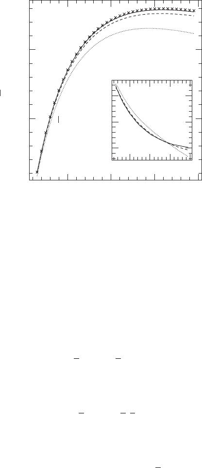
Figure 6.12 The rest mass

of a spherical n = 1 polytrope as a function of a density parameter q for three

different grid resolutions h (dotted line), h/2 (dashed line) and h/4 (solid line), computed with a code that solves

elliptic equations in three dimensions for quasiequilibrium binaries. The crosses mark the high-accuracy solution

obtained by solving the Oppenheimer–Volkoff ordinary differential equations for an equilibrium star in

spherical symmetry. The inset shows the rescaled numerical errors, which clearly converge to a single line,

establishing second-order convergence of the code. [From Baumgarte et al. (2004).]

Interestingly, neither an analytical nor a semi-analytical solution is needed to test the

convergence of a code. In a self-consistent convergence test we can eliminte the unknown

analytical solution u(t, x)in(6.152) by subtracting (6.153)

− u

h/2

+ O(h

). (6.157)

We similarly ﬁnd

4(u

h/2

− u

h/4

) =

+ O(h

). (6.158)

The higher-order error terms again keep decreasing, and the rescaled differences approach

h/k

(t, x) − u

h/(2k)

(t, x)) →

. (6.159)

This means that we can again check the convergence of our code, but this time completely

independently of any analytical solution. Clearly, this is a very powerful tool. Often we

can use the convergence to an analytical solution to test codes in certain regimes for which

an analytical solution can be found. But these tests may or may not test all aspects of

the computational algorithm. Self-consistent convergence tests, on the other hand, can be

228 Chapter 6 Numerical methods

used to test all parts of a code. The one down-side of a self-consistent convergence test,

compared to the convergence to an analytical solution, is that we now need at least four

different grid resolutions, so that we can form three pairs whose convergence we can test.

Exercise 6.25 Sometimes it is useful to “invent” an analytic solution where none

is known in order to perform a convergence test on a code. Consider the nonlinear,

ﬂat-space elliptic equation (6.54) for the function f (r):

∇

f = f

g, (6.160)

subject to boundary conditions

∂

f = 0, r = 0, (6.161)

∂

(rf) = 0, r =∞, (6.162)

where r

= x

+ y

+ z

.Taken = 4 for deﬁniteness. Here we will write and test a

code to solve this equation in one dimension (spherical symmetry), two dimensions

(axisymmetry), or three dimensions.

(a) Choose the arbitrary analytic function

f =

1 + r

, (6.163)

constructed to satisfy the boundary conditions, substitute it into equation (6.160)

and solve for g. Given this analytic source function g we now have an exact solution

f to equation (6.160) that satisﬁes the appropriate boundary conditions.

(b) Use the analytic source function g derived in part (a) to solve equation (6.160)

by ﬁnite-differencing. You may need to linearize the equation ﬁrst, as discussed at

the end of Section 6.2.2, and iterate the solution.

solution. Does your code converge at the expected convergence rate?

We also point out that any typo or mistake in an analytic equation that propagates into a high-order code will not be

discovered by a self-consistent convergence test. Only by comparison with an analytic solution can a convergence test

alone reveal such an error.

Locating black hole horizons

Black holes are characterized by the horizons surrounding them. Clearly, then, the numer-

ical simulation of black holes requires the ability to locate and analyze black hole horizons

in numerically generated spacetimes. In this chapter we ﬁrst review different concepts of

horizons in asymptotically ﬂat spacetimes, and then discuss how these horizons can be

probed numerically.

7.1 Concepts

Several different notions of horizons exist in general relativity. The deﬁning property

of a black hole is the presence of an event horizon (Section 7.2), but, as we will

see, apparent horizons (Section 7.3) also play an extremely important role in the con-

text of numerical relativity. In addition, the concepts of isolated and dynamical hori-

zons (Section 7.4) serve as useful diagnostics in numerical spacetimes containing black

holes.

A black hole is deﬁned as a region of spacetime from which no null geodesic can escape

to inﬁnity. The surface of a black hole, the event horizon, acts as a one-way membrane

through which light and matter can enter the black hole, but once inside, can never escape.

It is the boundary in spacetime separating those events that can emit light rays that can

propagate to inﬁnity and those which cannot. More precisely, the event horizon is deﬁned

as the boundary of the causal past of future null inﬁnity.

It is a 2 + 1 dimensional

hypersurface in spacetime formed by those outward-going, future-directed null geodesics

that neither escape to inﬁnity nor fall toward the center of the black hole. The event horizon

is a gauge-invariant entity, and contains important geometric information about a black

hole spacetime.

The intersection

H of the event horizon with a t = constant spatial hypersurface ,

i.e., the spatial “snapshot” of the horizon at the instant of time associated with ,forms

a closed, two-dimensional surface, whose proper surface area we denote as

A.Thearea

theorem

of classical general relativity states that this surface area can never decrease in

time,

A ≥ 0, (7.1)

See, e.g., Hawking and Ellis (1973); Wald (1984).

Hawking (1971, 1972, 1973).

229

230 Chapter 7 Locating black hole horizons

as long as all matter satisﬁes the null energy condition.

In the collision and coalescence

of two or more black holes, the surface area of the remnant black hole must be greater than

the sum of the progenitor black holes.

The fact that the event horizon area cannot decrease motivates the deﬁnition of the

irreducible mass

irr

≡



16π



1/2

. (7.2)

It is possible to extract energy and angular momentum from a rotating Kerr black hole.

While such an interaction can reduce the black hole’s mass, it cannot reduce its area,

according to the area theorem. The deﬁnition (7.2) then implies that the irreducible mass

of the black hole cannot decrease, which motivates its name.

Exercise 7.1 Verify that for a Schwarzschild black hole the irreducible mass M

irr

is equal to the ADM mass M

ADM

The area theorem can be used to place a strict upper limit on the amount of energy that

is emitted in gravitational radiation in black hole collisions.

Exercise 7.2 Consider two widely separated, nonrotating black holes of masses M

and M

, initially at rest with respect to some distant observer. Use the area theorem

to ﬁnd an upper limit on the energy emitted in gravitational radiation that arises from

the head-on collision of the two black holes. Verify that for equal mass black holes

at most 29% of the total initial energy can be emitted in gravitational radiation.

In Chapter 13 we will ﬁnd that considerably less energy is emitted in collisions of black

holes than the upper limit allowed by the area theorem.

Given the irreducible mass M

irr

and the angular momentum J of an isolated, stationary

black hole, we can compute the Kerr mass M (= M

ADM

) from

= M

irr

. (7.3)

Solving for M

irr

we ﬁnd

irr





1 +

)

1 −





, (7.4)

which implies that we have M

irr

≤ 2 for Kerr black holes, with equality in the extreme

Kerr limit when J = M

While the event horizon has some very interesting geometric properties, its global nature

makes it very difﬁcult to locate in a numerical simulation. The reason is that knowledge of

The null energy condition requires that T

≥ 0 for all null vectors k

. For a perfect gas, this condition requires

ρ + P ≥ 0.

Christodoulou (1970); Christodoulou and Rufﬁni (1971); see also Chapter 1.2.