Baumgarte T., Shapiro S. Numerical Relativity. Solving Einstein’s Equations on the Computer

Подождите немного. Документ загружается.

7.4 Isolated and dynamical horizons 251

in the surface element with s

, so that we can compute the angular momentum directly

in terms of 3 + 1 quantities.

Having deﬁned the angular momentum J

, it can be shown that the horizon mass is

given by



+ 4J

, (7.75)

where R

= (A

/4π)

1/2

is the areal radius of the horizon. This result is identical to that

found for Kerr black holes, but derived independenly within the framework of dynamical

horizons.

It is also possible to derive thermodynamic laws, and to relate the changes in horizon

mass and angular momentum between two intersections S

and S

of H to the matter and

radiation ﬂux across H between S

and S

Now turn to isolated horizons. When no more matter or radiation fall into the black

hole, the outgoing null vector k

becomes tangent to H, which is now a null surface. The

induced metric on H is then degenerate;

in fact, we may view the 2-metric m

induced

on the horizon S (see equation 7.14) as a degenerate 3-metric on H .

Since k

is tangent to H , equation (7.25) implies that the horizon area,

(

1/2

x, (7.76)

must remain constant. Several other interesting properties follow, and in particular we can

still measure the angular momentum and mass as in equations (7.74) and (7.75).

In anticipation of boundary conditions that we will use for the numerical construction

of initial data for black holes in equilibrium or quasiequilibrium (see Chapter 12.3)we

shall discuss one additional property of isolated horizons in more detail. By construction,

the expansion  vanishes everywhere on H. For isolated horizons, k

is tangent to H,so

we must also have

 = 0. (7.77)

Before we proceed it is useful to deﬁne the projection of the gradient of k



= m

∇

. (7.78)

We now decompose 

into its trace, symmetric-trace-free and antisymmetric parts as



 m

+ σ

+ ω

, (7.79)

Ashtekar and Krishnan (2003).

We call a metric q

induced on a surface H degenerate if it has a degenerate direction, meaning that there

exists a vector X

tangent to H so that q

= 0. A surface H is null if the metric induced on the surface is

degenerate.

252 Chapter 7 Locating black hole horizons

where

 = m



(7.80)

is the expansion scalar, with which we are well acquainted by now,

= 

(ab)

−

 m

(7.81)

is the shear tensor, and

= 

[ab]

(7.82)

is the rotation tensor.

Raychaudhuri’s equation applied to null geodesics with tangent vectors k

gives

 =−



− σ

+ ω

− R

. (7.83)

As we have discussed, on isolated horizons both  and

 vanish. Since the vectors k

are hypersurface orthogonal the rotation tensor ω

also must vanish.

Invoking Einstein’s

equation on the horizon in the absence of matter, we see that the last term in equation (7.83)

must be zero as well. That leaves σ

= 0, which implies the relation

= 0 (7.84)

on isolated horizons. As we will see in Chapter 12.3.2, this property of isolated hori-

zons will provide a boundary condition for the numerical construction of black holes in

(quasi)equilibrium.

See equation (2.39) in Section 2.4.3 of Poisson (2004).

See exercise 2.10 and Section 2.4.3 in Poisson (2004).

Spherically symmetric

spacetimes

Turn now from the most general spacetime in full 3 + 1 dimensions to the special case

of spherical symmetry. Why should we do this? Actually, spherical systems provide very

useful computational, physical and astrophysical insight and working with them serves

multiple purposes. The ﬁeld equations reduce to 1 +1 dimensions – variables may be

written as functions of only two parameters, a time coordinate t and a suitable radial

coordinate r – and are much simpler to solve in spherical symmetry. Solving them is a

very cost-effective way of probing dynamical spacetimes with strong gravitational ﬁelds,

including spacetimes with black holes. After all, nonrotating stars and black holes are

themselves spherical, so many important aspects of gravitational collapse, including black

hole formation and growth, can be studied in spherical symmetry. For example, the numer-

ical study of spherically symmetric collapse to black holes led to the discovery of critical

phenomena in black hole formation. The simpliﬁcation in the equations, together with the

reduction in the number of spatial dimensions, means that the system of spherical equations

can be solved more quickly, in terms of both human input and computer time, and with

much higher accuracy, than the set required for more general spacetimes. As a result, tack-

ling problems in spherical symmetry provides an excellent starting point for learning how

to do numerical relativity. It also serves as a convenient laboratory for experimenting with

different gauge choices (coordinates) and for generating high precision, test-bed solutions

for numerical codes designed to work in higher dimensions.

Having said all of this, we must bear in mind that there are important features of

dynamical spacetimes that will be missed when we restrict our attention to spherical

symmetry. Rotation cannot be treated in spherical symmetry. Spinning stars, star clusters

and black holes, rotational instabilities in stars and star clusters, relativistic effects induced

by the dragging of inertial frames – none of these features are present in spherical symmetry.

Moreover, gravitational radiation cannot be generated in spherical spacetimes: Birkhoff’s

theorem forbids it. We thus will have to postpone studying rotation and gravitational wave

generation until we relax the restriction to spherical symmetry and advance to axisymmetry.

In axisymmetry, spacetime has 2 + 1 dimensions – two spatial coordinates, e.g., r and a

polar angle θ,plust are necessary to specify the value of any function. Axisymmetry

253

254 Chapter 8 Spherically symmetric spacetimes

represents the lowest dimensionality at which rotation and gravitational radiation arise in

asymptotically ﬂat spacetimes.

The reduction in the number of degrees of freedom characterizing a spherical space-

time is reﬂected in the reduced number of nontrivial components of the 3-metric γ

that

must be determined by solving the 3 + 1 equations. In general, there are six indepen-

dent components of γ

: one component can be accounted for by the conformal factor

ψ, which is ﬁxed by the Hamiltonian constraint (e.g., equation 3.37), leaving ﬁve com-

ponents of the conformal 3-metric ¯γ

. Three of these components are related to the

three spatial coordinates and may be removed altogether by a suitable choice of the com-

ponents of the shift 3-vector β

. The remaining two components characterize the two

dynamical degrees of freedom associated with a gravitational ﬁeld, namely, the two polar-

ization states of a gravitational wave. Axisymmetric systems with rotation may give rise

to both dynamical degrees of freedom. However, if such a system happens to be stationary

and nonradiating, like a Kerr black hole or a rotating equilibrium star, neither of these

dynamical degrees of freedom are present. Axisymmetric systems without rotation can

possess only one gravitational degree of freedom. Moreover, if such a system is static

and nonrotating, as in the case of an oblate equilibrium star cluster, none are present.

In spherical symmetric spacetimes, neither dynamical degrees of freedom are allowed,

ever. The spacetime is nonradiating no matter how violently it may be changing with

time.

Choices! Choices!

The high degree of symmetry permits us to write the 3-metric of a spherical spacetime in

the general form

= Adr

+ Br

(dθ

+ sin

θdφ

), (8.1)

where A and B are functions only of t and r. To specify the full spacetime 4-metric we

also require the gauge functions α(t, r)andβ

(t, r). As we discussed above, we really

require only one nontrivial 3-metric coefﬁcient to ﬁx the 3-geometry.

Butwehavethe

gauge freedom inherent in our choice of the radial shift function β

(t, r) to cast the spatial

3-metric in alternative forms. There are a couple of different strategies we could adopt in

choosing the shift, as we discussed in Chapter 4.4. On the one hand, we could use the shift to

Both rotation and gravitational wave generation can arise in 1 + 1 dimensional spacetimes describing inﬁnite,axisym-

metric cylinders; see, e.g., Piran (1979) for a discussion and references. Plane gravitational waves of inﬁnite extent

can propagate in 1 + 1 dimensional spacetimes with planar symmetry; see, e.g., Bondi et al. (1959)andEhlers and

Kundt (1962) for some exact solutions and Centrella and Wilson (1983, 1984)andAnninos et al. (1989) for numerical

simulations.

Actually, we know from the Painlev

e–Gullstrand metric for a Schwarzschild spacetime (see Table 2.1) that we can have

A = B = 1, so that no nontrivial components are needed to specify the 3-metric in some cases.

Chapter 8 Spherically symmetric spacetimes 255

reduce the number of nontrivial 3-metric functions to the minimum required number, one.

Thus we could set B = 1inequation(8.1), in which case the radial coordinate r is the areal

or circumferential radius commonly referred to as the Schwarzschild radial coordinate:

r = r

= (A/4π )

1/2

= (C/2π ), where A is the proper area and C is the circumference

of a sphere centered at r

= 0. This is the “radial gauge” of Chapter 4.4. Alternatively,

we could set A = B,wherebyr =

r is an isotropic radial coordinate and we have the

“isotropic gauge”. The later choice also serves to globally minimize the distortion on the

grid, and is a special case of the minimum distortion gauge condition, as discussed in

Chapter 4.5. On the other hand, we could employ the shift vector to accomplish a different

task, like simplifying the matter ﬁeld rather than the gravitational ﬁeld. For example, we

might use the shift to maintain comoving coordinates, whereby the matter remains at rest

with respect to the spatial coordinates, with its 4-velocity satisfying u

∝ (∂/∂t)

at all

times.

Finally, we could simply get rid of the radial shift altogether, setting β

= 0. While

this may appear to be a simpliﬁcation, the price we pay is that we must now solve for both

A and B, except in special cases where (∂/∂t)

is a Killing vector and the metric functions

do not change with time.

Given everything we have discussed so far, we still have left the freedom to choose

the lapse function α to specify the time slicing. We could simply set α = 1, but we have

seen in Chapter 4.1 that such a choice (“geodesic slicing”) often leads to fatal coordinate

singularities in a numerical simulation. The appearance of a black hole raises a special

concern: the computational domain must avoid the physical (curvature) singularity inside

the hole at all costs, least the metric functions blow up and cause the code to crash before

the evolution is complete. One way to accomplish this is to choose a geometric “singularity

avoiding” lapse function, like maximal slicing or polar slicing. Another way is to choose

a “horizon penetrating” lapse condition that enables our spatial hypersurfaces to cross

the apparent horizon without encountering coordinate singularities in any of the metric

functions. That way we can employ black hole excision techniques, removing the central

singularity of the black hole and the surrounding neighborhood from the computational

domain altogether and replacing it, if needed, with a simple boundary condition at or

just inside the apparent horizon, where the metric is well-behaved. Yet another approach

employs the “moving puncture” method and gauge conditions, which we will discuss in

greater detail in Chapter 13.1.3.

All of the gauge choices discussed above have been utilized numerically at one time or

another. Several of them will be explored in the examples which follow, where we will

solve Einstein’s equations in 1 + 1 dimensions to construct spherical spacetimes. We will

begin with the simplest nontrivial spacetime – a single, isolated Schwarzschild black hole –

and work our way through some more complicated examples.

See Taub (1978), Section 15, for a shift prescription that maintains comoving coordinates for ﬂuids in arbitrary

dimensions and Eardley and Smarr (1979) for some numerical examples involving dust in spherical symmetry.

256 Chapter 8 Spherically symmetric spacetimes

8.1 Black holes

Here we shall construct the spacetime for a nonrotating, vacuum black hole by solving

the 1 + 1 equations. Starting from the same initial conditions, let us see how different

lapse and shift conditions lead to different foliations of spacetime. That is, let us see how

the resulting t = constant spatial slices differ, both in their “upward” climb in a spacetime

diagram, which measures the rate at which proper time as measured by a normal observer

advances from one slice to the next at different spatial locations, and in their “lateral”

extent, which measures the degree to which the slicing covers the interior of the black hole

at any time.

Familiar gauge choices

Before we solve the 1 + 1 equations formally to construct some examples of spherical

black hole spacetimes, let us anticipate the results we should rediscover if we adopt a few

familiar, analytic gauge conditions for α and β

together with suitable initial data. In all of

these examples, the lapse and shift form a Killing lapse and shift, as discussed at the end

of Chapter 2.7, so that all metric functions remain independent of time.

Begin with a case for which we specify the initial data on the time-symmetry slice

in the Kruskal–Szekeres diagram (see Figure 1.1): the spacelike v = 0 surface covering

0 ≤ u ≤∞in the u − v plane, or, equivalently, the t

= 0 slice from 2M ≤ r

≤∞in

standard Schwarzschild time and radial coordinates, t

and r

. Then we know that the

familiar gauge choice

α(r

) =

(

1 − 2M/r

)

1/2

,β

) = 0, (8.2)

gives the usual static solution for the 3-metric in Schwarzschild coordinates,

A(r

) =

1 − 2M/r

, B(r

) = 1. (8.3)

Slices of t

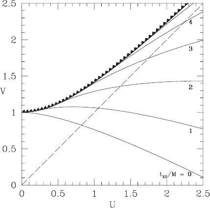
= constant in this foliation are shown in Figure 8.1.

The limiting slice asymptotes to the event horizon at r

= 2M as t

→∞; no slice ever

penetrates the horizon. Thus, standard Schwarzschild time slicing is singularity avoiding

but it is not horizon penetrating. A simple radial coordinate transformation can be used to

express this solution in terms of an isotropic radial coordinate

α(

r) =

1 − M/2

1 + M/2

,β

(

r) = 0, (8.4)

whereby

r) = B(

r) =



1 +



. (8.5)

This is not a different foliation, but rather the same time slicing as Schwarzschild, only

expressed in terms of a different radial coordinate.

8.1 Black holes 257

2.5

1.5

0.5

0 0.5 1

1.5 2 2.5

/M = 0

/M = 1.5

/M = 2

/M = 5

/M = 4

/M = 3

= 2

= 1

= 0

/M = 2.5

/M =

∞

/M = 3

Figure 8.1 Slices of constant Schwarzschild time t

for a spherical black hole, plotted in a Kruskal–Szekeres

diagram. The dashed line denotes the event horizon at r

/M = 2 and the sawtooth curve denotes the central

singularity at r

/M = 0.

By contrast with Schwarzschild time slicing, Kerr–Schild (or ingoing Eddington–

Finkelstein) slicing is horizon penetrating, but it is not singularity avoiding. These proper-

ties make Kerr–Schild slicing (or a lapse condition close to it), a good candidate for black

hole excision. As in the case of Schwarzschild, the Kerr–Schild solution is analytic and

static. However, none of the Kerr–Schild t

= constant slices are time-symmetric, since

the diagonal components of K

) never vanish. So we cannot expect the time-symmetric

slice in the Kruskal–Szekeres diagram to provide initial data for this solution. Instead, we

need data on a t

= constant slice, any one of which will sufﬁce, since the 3-geometry is

still static in this time coordinate. The Kerr–Schild gauge conditions are

α(r

) =



+ 2M



1/2

,β

) =

+ 2M

. (8.6)

and the 3-metric for this solution is given by

A(r

) = 1 +

, B(r

) = 1. (8.7)

To locate the t

= constant time slices on a Kruskal–Szekeres diagram we need to express

u and v as functions of t

and r

in regions I and II of the diagram. We ﬁnd, up to an

arbitrary additive constant absorbed in t

u =

)/4M

+ e

−r

)/4M

/2M − 1)

v =

)/4M

− e

−r

)/4M

/2M − 1)

(8.8)

258 Chapter 8 Spherically symmetric spacetimes

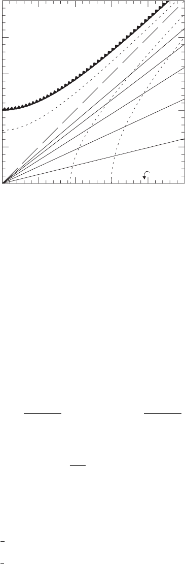
Figure 8.2 Slices of constant Kerr–Schild (ingoing Eddington–Finkelstein) time of a Schwarzschild black hole,

plotted on a Kruskal–Szekeres diagram. The dashed line denotes the event horizon at r

/M = 2 and the sawtooth

curve denotes the central singularity at r

/M = 0.

Exercise 8.1 Verify equation (8.8). Begin by matching the Schwarzschild and

Kerr–Schild line elements to show that

= t

+ 2M ln |r

/2M −1|+C, (8.9)

where C is a constant which can be set equal to zero. Then use this equation together

with the transformations between Kruskal–Szekeres and Schwarzschild coordinates,

in regions I and II of the Kruskal–Szekeres diagram,

/2M −1)e

/2M

= u

− v

(8.10)

and



4M tanh

−1

(v/u), in region I, r

> 2M,

4M tanh

−1

(u/v), in region II, r

< 2M,

(8.11)

to derive

= 4M ln(u + v) − r

, (8.12)

which holds in both regions. Finally, use equations (8.10)and(8.12)toderive

equation (8.8).

Using equation (8.8), we plot slices of constant t

in Figure 8.2. We see from the ﬁgure

that all of the slices penetrate the horizon, and all of them hit the central singularity. So

Kerr–Schild time slicing is horizon penetrating but not singularity avoiding. This time

slicing, and slicings with lapse functions close to it, provide a good gauge for performing

black hole excision.

8.1 Black holes 259

Maximal slicing

Maximal slicing has the advantage that it is both horizon penetrating and singularity

avoiding. As a result, it has been adopted in many numerical simulations involving black

holes. Typically, imposing the maximal slicing condition does not admit an exact solution to

the 1 + 1 equations. Remarkably, for the case of a single, nonrotating black hole in the radial

gauge, analytic solutions for a maximal spacetime do exist, even in the presence of a radial

shift. We already derived an entire family of time-independent solutions in Chapter 4.2

(see equations 4.23–4.25). Here we will construct another maximal slicing of the same

spacetime, one that gives a time-dependent or “dynamical slicing” of a Schwarzschild

black hole.

This spacetime is also analytic, if by “analytic” we allow 1-dimensional

quadratures. The metric for this solution has some generic features that characterize the

metric that develops at late times during stellar collapse to a black hole when maximal

slicing is employed. Not only will our examination of this solution be useful to illustrate

how maximal slicing works, but our reconstruction of the solution will provide a convenient

opportunity to review the typical steps required to build a spacetime in the 3 + 1 formalism,

at least in spherical symmetry.

We start with the line element in the form

=−(α

− β

/A)d

+ 2βd

tdr + Adr

(dθ

+ sin

θdφ

), (8.13)

where r is the Schwarzschild radial coordinate (we drop the subscript “s” in this section),

β = β

= Aβ

t is the maximal time coordinate, and the functions α, β and A depend

only on

t and r . Given this form of the metric we compute all the 3-dimensional Christoffel

symbols, which we will need in the evaluation of the standard 3 +1 or ADM equations.

We ﬁ nd



= ∂

A/(2A),

θθ

=−r/A,

φφ

=−r sin

θ/A,



rθ

= 

θr

= 1/r,

φφ

=−sinθ cosθ, (8.14)



θφ

= 

φθ

= cotθ, 

rφ

= 

φr

= 1/r,

with the remaining coefﬁcients equal to zero.

Exercise 8.2 For practice, obtain the Christoffel symbols displayed in equa-

tion (8.14) by employing the Lagrangian

L = A

sin

(8.15)

to write down the 3-dimensional Euler–Lagrange equations and then matching them

to the 3-dimensional geodesic equation

+ 

= 0, (8.16)

to get the nonvanishing symbols.

Estabrook et al. (1973); our discussion is patterned after their treatment.

260 Chapter 8 Spherically symmetric spacetimes

Next we insert the Christoffel symbols in equation (2.142) to calculate the nonvanishing

components of the 3-dimensional Riemann tensor, R

, obtaining

= ∂

A/(rA), R

θθ

= R

φφ

/sin

θ = 1 − 1/ A +r∂

A/(2A

). (8.17)

We now can get R = R

, required to solve the Hamiltonian constraint equation (2.132):

R = 2∂

A/(rA

) + 2(1 − 1/ A)/r

. (8.18)

The nonvanishing components of the extrinsic curvature may be calculated from equa-

tion (2.134), yielding

=−(∂

A + β∂

A/A − 2∂

β)/(2α), K

θθ

= K

φφ

/sin

θ = rβ/(α A). (8.19)

Maximal slicing requires K = K

= 0, in which case equation (8.19) implies

=−2β/(αr ), K

= 6(β/αAr)

(8.20)

and

−∂

ln A + (β/A)∂

ln(β

/A) = 0. (8.21)

The Hamiltonian constraint (2.132) reduces to

R = K

, (8.22)

which, inserting equations (8.18) and (8.20), yields

3β

/(α

A) = A − 1 +r∂

A/A. (8.23)

When combined with equation (8.20)forK

, the radial component of the momentum

constraint (2.133) may be evaluated to give

∂

ln(βr

/Aα) = 0. (8.24)

Maximal slicing also requires ∂

K = 0, in which case equation (2.137), combined with

equation (8.22), gives D

α = αR. Substituting equation (8.18) in the right-hand side and

expanding the derivative on the left-hand side yields an equation for the lapse,

∂

α + 2∂

α/r − (∂

ln A)∂

α/2 = 2α(A − 1 +r∂

ln A)/r

. (8.25)

Finally, the evolution equation (2.135)forK

gives

∂

ln(β/α) = (3β/A + α

A/β − α

/β)/r

+3(∂

β)/ A + (α

/β − 4β/A)(∂

ln A)/2 (8.26)

−(β/A + α

/β)∂

ln α,

wherewehaveusedequation(8.20) to replace K

, equation (8.17)forR

, and equation

(8.25)for∂

∂

α.