Baumgarte T., Shapiro S. Numerical Relativity. Solving Einstein’s Equations on the Computer

Подождите немного. Документ загружается.

8.3 Fluid stars: collapse 301

It is clear that very few modiﬁcations are needed to transform the Misner–Sharp equa-

tions to observer time coordinates. Hence a code using Misner–Sharp equations can be

rewritten in observer time coordinates simply by adding a few terms and using ψ instead

of φ. The advantage is that the revised code can handle black holes without breaking down.

There are two very attractive properties of observer time coordinates. One is that the

coordinate u immediately corresponds to the time at which a distant observer would see

a certain event, as for example a gamma-ray burst (GRB) in a supernovae explosion.

The other one is that the global structure of spacetime is conveniently “hard-wired” into

the integration scheme. This means that there is no need to search for apparent horizons

(actually, apparent horizons never appear in observer time coordinates because they are

always inside event horizons) or to track null rays in order to locate event horizons. In

this case the event horizon can be found simply by looking for events at the which the

lapse function e

becomes exceedingly small. The lapse function plummets for every ﬂuid

element approaching the event horizon and essentially causes its further evolution to cease.

For a typical application involving collapse to a black hole, one can terminate the evolution

if and when e

drops below, say 10

−3

at the outermost shell. By then, the lapse in the

center can be considerably smaller and can reach machine underﬂow.

The only subtlety that arises in using observer time coordinates has to do with the

implementation of initial data. It is usually convenient to specify initial data on a spatial

t = constant hypersurface instead of a null hypersurface. Consequently, for typical appli-

cations, the implementation of initial data occurs in two stages. First, initial data are given

on a t = constant surface. These are then evolved using a Misner–Sharp scheme. During

this evolution, a null geodesic is sent out from the center of the conﬁguration, and the

data on its path are stored. When the null ray arrives at the surface, this stage of the

evolution can be stopped and the data on the ray’s path can now be used as initial data on

a u = constant = 0 surface, at which point the Hernandez–Misner scheme takes over for

the rest of the evolution.

As an example of the Hernandez–Misner scheme at work, we show in Figure 8.21 “test-

bed” results for the collapse of a homogeneous, dust ball initially at rest, i.e., Oppenheimer–

Snyder (OS) collapse. As we noted earlier, OS collapse provides one of the few highly

nonlinear, dynamical examples in general relativity for which the solution is known ana-

lytically (see Chapter 1.4). However, as we noted in previous cases, before this analytic

solution can be compared with the numerical results, the solution must be transformed to

the coordinate system adopted in the numerical approach. This transformation has been

carried out

for null coordinates and the comparison with a numerical simulation in these

coordinates is shown in the ﬁgure.

A more interesting result is shown in Figure 8.22 for the collapse of a 1.4M



, n = 3

polytrope with adiabatic index γ = 4/3 and initial central density ρ

= 10

gcm

−3

Plotted in the ﬁgure is a spacetime diagram for the late time evolution of a conﬁguration in

Baumgarte et al. (1995).

302 Chapter 8 Spherically symmetric spacetimes

10.9

10.8

10.7

10.6

τ /M

0.5

0.45

0.35

0.3

0.4

0.3

0.2

0.1

0.01

0.001

2.052

R/MR/M

R/M

R/M R/M

R/M

2.1

1.95 2

2 2.051.951.9

2.05 2.1

u=4

u=6

u=10

u=6

u=7

u=8

Figure 8.21 Oppenheimer–Snyder collapse of a star with initial compaction R/M = 5. Shown are a spacetime

diagram with worldlines of selected mass shells (top row), rest-density proﬁles (middle row) and lapse function

proﬁles (bottom row) at different observer times u. The analytic solution is represented by solid lines (worldlines

of mass shells) and dotted lines (lines of constant u), while numerical results are represented by dots. [From

Baumgarte et al. (1995).]

which the initial pressure was slightly reduced everywhere by a factor d = 0.9946 below

the equilibrium value at t = 0.

In general relativity, all spherical equilibrium stars with

γ = 4/3 are unstable to radial collapse,

so it is not surprising that the star undergoes an

implosion. This case serves as a crude model for core collapse in a nonrotating, massive star

at the endpoint of stellar evolution (at least prior to reaching nuclear densities). By simply

This case was ﬁrst studied by van Riper (1979).

See, e.g., Shapiro and Teukolsky (1983), Chapter 6.9.

8.4 Scalar ﬁeld collapse: critical phenomena 303

780

775

770

765

1 10 100

R/M

t[ms]

Figure 8.22 Comparison of simulations of the collapse of a slightly pressure-depleted 1.4M



core with

= 10

gcm

−3

and γ = 4/3. Plotted is a spacetime diagram of the late-time evolution showing the worldlines

of Lagrangian mass shells obtained with a Hernandez–Misner code (solid lines) and a Misner–Sharp code

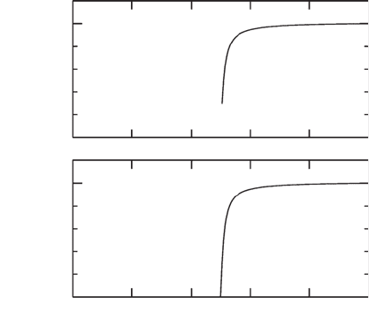
(crosses). The dashed line marks the event horizon. [From Baumgarte et al. (1995).]

rescaling the mass, the calculation also provides a good model for the collapse of a radially

unstable, nonrotating, supermassive star.

Results are shown both for a Misner–Sharp

simulation and a Hernandez–Misner simulation. The agreement in the time of collapse is

within 0.05%. We note, however, that the Misner–Sharp simulation penetrates the event

horizon and breaks down shortly after the formation of an apparent horizon, while the

Hernandez–Misner simulation covers the entire spacetime outside the event horizon.

8.4 Scalar ﬁeld collapse: critical phenomena

Initial data sets for relativistic collapse typically divide themselves into two groups: those

that lead to black hole formation and those that do not. One of the most important triumphs

of numerical relativity has been the discovery by Choptuik that at the threshold of black hole

formation, gravitational collapse solutions in general relativiy exhibit “critical behavior”.

Speciﬁcally, collapse solutions for initial data at black hole threshold exhibit universality,

In core collapse of a massive star, the EOS is dominated by relativistic, degenerate electrons above nuclear densities,

while in a supermassive star, the EOS is dominated by thermal radiation pressure. In both cases, γ ≈ 4/3.

For more realistic examples of stellar core collapse employing the Hernandez–Misner formulation, including neutrino

emission, see Baumgarte et al. (1996).

Choptuik (1993); as reported here, the discovery came about as the direct result of a question posed to Choptuik in

1987 by Christodoulou: “will black hole formation turn on at ﬁnite or inﬁnitesimal mass for a generic interpolating

family at threshold?”

304 Chapter 8 Spherically symmetric spacetimes

scaling and self-similarity in analogy with critical behavior in statistical mechanics. The

existence of such “critical phenomena” are interesting for revealing the surprising structure

and simplicity that underlies collapse solutions in general relativity and for providing

insight into cosmic censorship and the dynamical character of Einstein’s ﬁeld equations.

Following their discovery, critical phenomena have been pursued by numerous numerical

simulations and also by perturbation treatments which utilize the formalism and techniques

of dynamical systems theory and the renormalization group.

Remarkably, critical phenomena can be explored in some detail by working with one

of the simplest examples of gravitational collapse: the implosion of a massless scalar

ﬁeld in spherical symmetry. In fact, it was this model that was probed by Chopuik in his

original analysis. The existence of critical behavior in such a system arises from the generic

competition between two dynamical effects: the kinetic energy of the ﬁeld, which tends to

disperse it to inﬁnity, and its gravitational potential energy, which, if sufﬁciently strong,

can trap some of the mass-energy in a black hole. Choptuik realized that for any family

of initial data, the dynamical competition could be controlled by tuning a parameter in the

initial conditions (e.g., the amplitude of the initial ﬁeld). If the parameter p is less than

some critical (threshold) value p

∗

, the scalar ﬁeld disperses completely, while if p > p

∗

a black hole forms.

To examine quantitatively what happens for p in the neighborhood of p

∗

, we ﬁrst need

to evolve the system numerically. Toward this end, we assemble the full set of equations for

evolving a massless scalar ﬁeld in spherical symmetry in the next section. This is a good

exercise in working with the equations of numerical relativity and then applying them to

address a fundamental physics issue.

Basic equations

Suppose we start with the spherical metric in the form given by equation (8.13). Here r is

the areal coordinate, whereby the surface area of a 2-sphere of constant t and r is 4πr

Adopt polar time slicing, for which

K = K

, K

= K

= 0. (8.129)

According to equation (8.19), the requirement of polar slicing implies β = 0, i.e., the shift

must be zero everywhere. Setting A = a

we can thus cast the metric in the simple diagonal

form

=−α

(t, r)dt

+ a

(t, r)dr

(dθ

+ sin

θ dφ

), (8.130)

which serves as the starting point of Choptuik’s analysis. We need to ﬁnd two ﬁeld equations

to determine the two functions α and a in the metric. We can obtain an equation for a from

For excellent reviews and references, see Gundlach (2000, 2003)andChoptuik (1998), from which much of the

discussion in this section is drawn

8.4 Scalar ﬁeld collapse: critical phenomena 305

the Hamiltonian contraint, equation (2.132), which simpliﬁes to R = 16πρ in the adopted

slicing, since K

= K

. Using equation (8.18)toevaluateR,wearriveat

− 1

= 4πρra

. (8.131)

The slicing condition ∂

θθ

= 0 yields the equation for α. Using equation (2.135), we may

write

0 = ∂

θθ

= α R

θθ

− D

α − 8πα

θθ

−

(S − ρ)

. (8.132)

Using equation (8.17)toevaluateR

θθ

, and using D

α = r∂

α/a

, yields the desired

equation for α,

dα

−

− 1

=−8π

θθ

−

(S − ρ)

. (8.133)

The matter source is given by the stress-energy tensor for a massless, noninteracting, real

scalar ﬁeld,

=∇

ϕ∇

ϕ −

∇

ϕ (8.134)

(cf. equation 5.232). Deﬁning the auxiliary scalar ﬁeld variables  and  according

(t, r) ≡ ∂

ϕ(t, r ), (8.135)

(t, r) ≡

∂

ϕ(t, r ), (8.136)

and referring to equation (2.138), we can express the matter source terms as

follows:

ρ = (

+ 

)/(2a

), (8.137)

=−()/a, (8.138)

= ρ, (8.139)

= S

= (

− 

)/(2a

), (8.140)

S = (3

− 

)/(2a

). (8.141)

The ﬁeld equations (8.131) and (8.133) thus reduce to

− 1

− 2πr (

+ 

) = 0, (8.142)

dα

−

− 1

= 0. (8.143)

306 Chapter 8 Spherically symmetric spacetimes

Exercise 8.17 Derive an evolution equation for a. Use equation (8.19)forK

together with the momentum constraint (2.133), to show

∂

a = 4πrα. (8.144)

It is thus not necessary to solve any evolution equations for the gravitational ﬁeld, like

equation (8.144), but instead one can integrate the ﬁrst order ODE equations (8.142)and

(8.143), (really radial quadratures), at each new time slice. Such a “constrained” scheme

typically produces a more stable and accurate integration; equation (8.144) will be satisﬁed

automatically. The matter ﬁeld, however, must be evolved. The equation of motion is the

massless Klein–Gordon equation (5.235). In terms of the auxiliary variables, this wave

equation may be cast as two ﬁrst-order equations,

∂

 = ∂







, (8.145)

∂

 =

∂







. (8.146)

Exercise 8.18 Derive the two ﬁrst-order equations above.

A useful geometric diagnostic is the mass function m(t, r ) which in spherical symmetry

can deﬁned invariantly by

1 −

2m(t, r)

≡∇

r∇

r = a

−2

, (8.147)

(cf. exercise 8.9). In the limit r →∞, m approaches the ADM mass (=total mass-energy)

of the spacetime. As we have discussed, polar slices cannot cross apparent horizons.

However, black hole formation is deﬁnitely signaled by 2m/r → 1 at some areal radius

r = R

; at this radius, the mass of the ﬁnal black hole can be calculated from M

/2.

Boundary conditions on the ﬁeld and matter variables are now straightforward to specify.

Equations (8.142) and (8.143) can be integrated outward from r = 0, where we can set

a = 1andα = 1. The boundary value for a guarantees regularity at the origin according

to equation (8.147). The boundary value for α makes the coordinate time t the proper time

measured by a normal observer at the origin, which is a convenient parametrization of the

t = constant hypersurfaces. For the scalar ﬁeld, regularity at the origin requires ∂

ϕ = 0.

At large radii, where the spacetime is asymptotically ﬂat, we can impose outward spherical

wave boundary conditions, e.g., rϕ(t, r) = f (t −r) for some function f . An equivalent

way to write this condition is ∂

(rϕ) + ∂

(rϕ) = 0asr →∞, which is simple to impose.

Exercise 8.19 Translate the inner and outer boundary conditions on ϕ(t, r)to

boundary conditions on (t, r)and(t, r).

We have now assembled all of the relevant equations required in Choptuik’s original

analysis.

8.4 Scalar ﬁeld collapse: critical phenomena 307

(a) (b)

(d)(c)

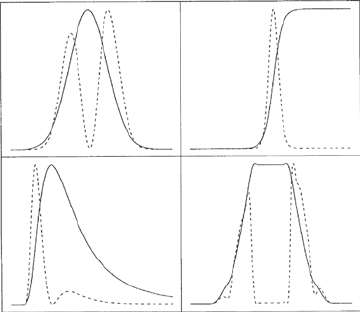
Figure 8.23 Typical initial proﬁles of the scalar ﬁeld ϕ (solid lines) and the radial mass-energy density dm/dr

(dotted lines) for four families of initial data considered by Choptuik. [From Choptuik (1993).]

Exercise 8.20 Show that the rescaling

t → kt, r → kr,ϕ→ ϕ,→ k

−1

,  → k

−1

, (8.148)

transforms one solution into another for any positive k.

Numerical results

Suppose we now consider one-parameter families of massless scalar ﬁeld initial data and

evolve them for many different values of the parameter p. For example, one of the many

families considered by Choptuik consisted of ingoing Gaussian wave packets ϕ(0, r) =

exp(−[(r − r

)/δ]

), with the parameter p taken variously to be the amplitude ϕ

,the

centroid r

, the width δ and the power-law q. A typical proﬁle is sketched in Figure 8.23.

Exercise 8.21 Consider the evolution of a massless spherical scalar ﬁeld in ﬂat

space for a speciﬁed initial packet ϕ(0, r). Derive the initial auxiliary scalar ﬁelds

(0, r)and(0, r) in terms of ϕ(0, r) by requiring that the initial data yield a purely

ingoing spherical wave.

Hint: Argue that the solution must be of the form ϕ(t, r ) = g(t +r)/r for some

function g(x).

The parameter p is a measure of the strength of the gravitational interaction. Strong

interactions (high p, say) lead to black hole formation; weak interactions (low p) do not

and lead to dispersal instead.

The critical transition value p

∗

is found empirically.

The ﬁrst signiﬁcant result to emerge from Choptuik’s study is that for generic fam-

ilies of initial scalar ﬁeld data, the black hole masses are well-ﬁt by the scaling

Christodoulou (1986, 1991, 1993) established that weak spherical scalar waves disperse and strong waves form black

holes and that these are the only two ﬁnal states.

308 Chapter 8 Spherically symmetric spacetimes

−1.0

−3.0

In f

− f

∗

In M

= 0.376

−5.0

−26.0 −22.0 −18.0

−14.0

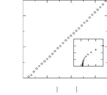
Figure 8.24 Typical evidence for mass scaling in the collapse of a spherical massless scalar ﬁeld. The initial

data consists of a one-parameter family of ingoing Gaussian pulses of scalar ﬁeld in which the amplitude ϕ

varied. The mass-scaling exponent, γ

≈ 0.376, is determined from a least-squares ﬁt. The inset shows that the

transition is Type II. For Gaussian initial data, the scaling persists well beyond the critical limit, p → p

∗

.[From

Choptuik (1998).]

relation

= C|p − p

∗

, (8.149)

where C is a constant that depends on the family but where the exponent γ is universal,

γ  0.37, independent of family. The evidence is displayed in Figure 8.24.

Black hole formation turns on at inﬁnitesimal mass in the case of a massless scalar ﬁeld,

and this situation is designated a Type II critical phenomenon. By contrast, in a Type I

transition, black holes ﬁrst appear at ﬁnite mass.

The designations are in analogy with

ﬁrst and second order phase transitions in statistical mechanics. The two possibilities are

distinguished schematically in Figure 8.25.

The second surprising result was the appearance of universality, the phenomenon

whereby for a ﬁnite length of time in a ﬁnite region of space, the spacetime generated

by all families of near-critical initial data approach the same solution. This universal crit-

ical solution to the equations of motion is approached by all initial data that are close to

black hole threshold, on both sides of the critical solution, for any one-parameter family.

The solution is determined up to an overall scale factor depending on the family. The

critical solution is obviously unstable, as the slightest perturbation will result either in

black hole formation or complete dispersal. When the evolution chooses one of the two

routes, the universal phase ends.

The third ﬁnding revealed by Chotpuik’s simulations is scale-echoing. This phenomenon

is a form of discrete self-similarity, whereby as one tunes closer and closer to the critical

The collapse of a massive scalar ﬁeld is a Type I phenomenon, as is the collapse of collisionless matter.

8.4 Scalar ﬁeld collapse: critical phenomena 309

0.0

weak

strong

1.0

0.0

(fraction of total)

Figure 8.25 Schematic illustration of possible black-hole threshold behavior. The top panel represents a Type I

(“ﬁrst-order”) transition, where the “order parameter” M

is nonzero at threshold. The bottom panel shows a

Type II (“second order”) transition, where M

is inﬁnitesimal at the critical point. [From Choptuik (1998).]

solution, the dynamical character of the solution repeats itself at ever-decreasing time and

length scales related by a factor of e



,where  3.44, so that e



 30. Mathematically,

the critical solution ϕ

∗

(t, r) and associated spacetime satisfy



= e

−n

t (8.150)



= e

−n

r (8.151)



= e

−2n

(8.152)

∗



, r



) = ϕ

∗

(t, r) (8.153)

(n = 1, 2, 3 ...). (8.154)

The dimensionless critical exponent γ and echo period  are two interesting constants

whose origins are still somewhat of a mystery.

The behavior discovered by Choptuik has been found in other forms of matter coupled to

gravity. It has even been demonstrated in the collapse of axisymmetric gravitational waves

in pure vacuum spacetimes.

The existence of the critical exponent and echo period

appears to be universal, but their values depend on the type of matter.

A signiﬁcant consequence of Type II critical solutions is that they produce naked

singularities: a critical solution results in a point of inﬁnite curvature which is visible to

observers at future null inﬁnity. For example, the spacetime scalar curvature

(4)

R grows

without bound near r = 0 in a precisely critical massless scalar ﬁeld evolution.

Abrahams and Evans (1993); γ ≈ 0.37, ≈ 0.6

310 Chapter 8 Spherically symmetric spacetimes

Exercise 8.22 Show that

(4)

R is easily evaluated for a massless scalar ﬁeld as

(4)

R = 8π ∇

ϕ∇

ϕ = 8π (

− 

)/a

. (8.155)

Thus Type II critical solutions provide counterexamples to the Cosmic Censorship

Conjecture,

which asserts that the collapse of well-behaved initial data does not result in

a naked singularity. While it is always possible to restate the conjecture so that it applies

only to the collapse of generic initial data, and thereby rule out these critical solutions

on technical grounds, these counterexamples do highlight why is has been so difﬁcult to

fashion a rigorous proof.

Penrose (1969).

See Berger (2002) for discussion and references; see also Chapter 10.1.