Baumgarte T., Shapiro S. Numerical Relativity. Solving Einstein’s Equations on the Computer

Подождите немного. Документ загружается.

12.4 Quasiequilibrium sequences 421

the helical Killing vector (12.63) is not an inertial observer. For a true stationary spacetime

we can split this helical Killing vector into separate rotational and timelike Killing vectors.

For binaries this split cannot be done globally, but, assuming asymptotic ﬂatness, the two

can be separated at spatial inﬁnity. There the timelike Killing vector deﬁnes an inertial

observer, and we see from the boundary condition (12.73) that the shift approaches the

rotational Killing vector

lim

r→∞

= β

rot

≡ 

orb



∂

∂φ



= (Ω

orb

× r)

. (12.109)

In general the latter makes a nonvanishing contribution to the Komar mass.

Exercise 12.11 Show that substituting β

rot

into the Komar mass integral (3.179)

yields a contribution

rot

=−2

orb

J, (12.110)

where J is the angular momentum (3.189).

Evaluating the Komar mass integral in the corotating frame, for which the shift behaves

according to (12.109), yields a value that differs from what we would ﬁnd in an inertial

frame by M

rot

corot

= M

inertial

− 2

orb

J. (12.111)

This raises the question: which one of these values are we supposed to compare with

the ADM mass M

ADM

in equation (12.108)? The expression (3.128) for the ADM mass

assumes that it is evaluated in an inertial frame, since otherwise the fall-off conditions

(3.129) would not be satisﬁed. Moreover, the Komar mass requires a timelike Killing

vector, and outside the “light cylinder” (on which ξ

hel

is null) the helical Killing vector

(12.63) becomes spacelike. This means that we have to evaluate the Komar mass in the

asymptotic inertial frame. Our conformal thin-sandwich calculation is performed in the

corotating frame, but we can account for that in one of three ways. If all “nonrotational”

contributions to the shift fall off sufﬁciently fast, we can simply ignore the shift term in the

integral (3.179) and compute the Komar mass from the lapse term alone (as many authors

do). If the nonrotational contributions to the shift cannot be ignored, we can subtract β

rot

before computing the Komar mass, or, equivalently, we can simply transform the Komar

mass computed in the corotational frame to its value in the inertial frame with the help of

equation (12.111).

12.4 Quasiequilibrium sequences

As we discussed in Section 12.1, we can model the early (adiabatic) binary inspiral

phase as a sequence of quasiequilibrium conﬁgurations. In the previous sections we have

For a discussion of the invariance of the integrals deﬁned in Chapter 3.5 for M

, M

ADM

and J

ADM

when they are

evaluated in the corotating vs. the inertial frame, see Duez et al. (2003), Appendix C.

422 Chapter 12 Binary black hole initial data

developed techniques for constructing black hole binaries with certain black hole masses,

spins and binary separations. Before we can stitch these together to construct evolutionary

sequences we have to address one more question: what are the conserved quantities along

these sequences?

For binary neutron stars it is quite evident that, in the absence of mass loss or accretion,

the rest-mass (e.g., baryon number) of each neutron star is strictly conserved during binary

inspiral (see Chapter 15.3). For binary black holes, identifying a conserved quantity is a

little more subtle. As long as the individual black holes remain in quasiequilibrium as they

evolve, it is reasonable to assume that their irreducible masses given by equation (12.60)

remain constant.

One approach to constructing an inspiral sequence is therefore to iterate, at a given

coordinate separation of the binary pair, over the individual masses until the desired

irreducible masses have been achieved. The procedure can then be repeated for different

binary separations, until a sequence has been completed. A more elegant approach utilizes

the relation

ADM

= 

orb

dJ, (12.112)

which strictly holds along stationary sequences of uniformly rotating conﬁgurations. We

have effectively encountered this relation as it applies to binaries in exercise 12.2 and

in the last part of exercise 12.4; it is the relativistic generalization of equation (12.14).

In exercise 12.12 we illustrate how equation (12.112) can be enforced when connecting

numerical models along a quasiequilibrium sequence.

Exercise 12.12 Let s denote some parameter along a sequence of binary black hole

initial data, and let χ (s) denote an arbitrary length scale along this sequence. Also

write the ADM mass, angular momentum and orbital frequency along the sequence

ADM

(s) = χ (s) e(s) J (s) = χ

(s) j(s) 

orb

(s) = χ

−1

(s) ω(s), (12.113)

where e(s), j(s)andω(s) are numerical values of these quantities in nondimensional

units. Show that the identity (12.112) is automatically satisﬁed as long as χ changes

according to

dχ

=−

de − ωdj

e − 2ωj

(12.114)

along the sequence.

Black hole perturbation theory suggests that the fractional increase in the surface area of each hole in a binary

consisting of equal-mass holes with spins aligned with the orbital angular momentum (and 99.8% of their maximal

values) is at most 1% by the time the binary spirals down to a separation of 6M,whereM is the total (ADM) mass;

Alvi (2001).

See Friedman et al. (2002). See also equation (14.25) and related discussion.

Cook and Pfeiffer (2004).

12.4 Quasiequilibrium sequences 423

l/M

−0.07

−0.06

−0.05

−0.04

−0.03

−0.02

Komar sequence

Minima of EP

4.5

3.9

4.3

4.1

3.7

3.65

3.60

3.55

3.50

3.45

3.40

3.38

3.35

3.30

/µ

l/M

−0.08

−0.07

−0.06

−0.05

−0.04

−0.03

−0.02

/µ

Komar sequence

Minima of EP

4.5

4.1

3.7

3.5

3.30

3.25

3.20

3.15

3.12

3.10

3.35

3.40

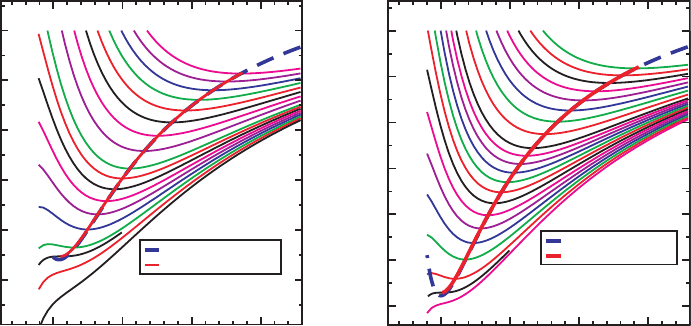
Figure 12.5 The binding energy E

vs. separation l for corotational (left panel) and nonspinning (right panel)

equal-mass binary black hole sequences constructed in the conformal thin-sandwich approach. The solid lines

connecting the extrema of the curves of constant angular momentum, which are labeled by J/µM,represent

sequences constructed with the effective potential method as in Figure 12.3; these lines terminate at the ISCO.

The dashed lines represent sequences constructed from the mass criterion (12.108). These sequences agree

extremely well up to very small separations, where the assumption of quasiequilibrium breaks down. [From

Caudill et al. (2006).]

We have already seen an example of such a sequence in Figure 12.3 for Bowen–

York binary data constructed with the transverse-traceless approach of Section 12.2.As

with the point-mass models that we discussed in Section 12.1 this sequence does not

extend to arbitrarily small binary separations, but instead terminates at the innermost

stable circular orbit, or ISCO, marked by the turning point on the equilibrium energy

curve.

In Figure 12.5 we show the equivalent ﬁgures for corotational and nonspinning binary

black hole models constructed in the conformal thin-sandwich approach of Section 12.3.

For most of the remainder of this section we will focus on the results of Cook and Pfeiffer

(2004)andCaudill et al. (2006), who adopt spectral methods to integrate these equations,

together with the quasiequilibrium black hole boundary conditions of Section 12.3.2. They

also assume conformal ﬂatness, ¯γ

= η

and maximal slicing K = 0, as well as

= 0

and ∂

K = 0.

Within this framework we can specify a corotational sequence by setting



spin

= 0 in the solution (12.107) for the black hole boundary condition on the tangential

piece of the shift.

Specifying an nonspinning sequence is slightly more involved. As

we discussed below equation (12.107), we could attempt to construct such sequences by

See Cook and Pfeiffer (2004) for some results that adopt “Kerr–Schild” slicing rather than maximal slicing.

Recall that 

spin

is a measure of the spin in the corotating frame.

424 Chapter 12 Binary black hole initial data

0.03

−0.04

−0.05

−0.06

−0.07

−0.08

−0.09

0.06

0.09 0.12

MΩ

orb

CO: MS -

CO: HKV - GGB

CO: EOB - 3PN

CO: EOB - 2PN

CO: EOB - 1PN

0.04 0.08 0.12

0.16

MΩ

orb

/µ

NS: - d(αψ)/dr = (ψψ)/2r

d(αψ)/dr = (ψψ)/2r

LN: - d(ψψ)/dr = (ψψ)/2r

NS: IVP Conf. Imaging/Eff. Pot.

NS: EOB - 3PN

NS: EOB - 2PN

NS: EOB - 1PN

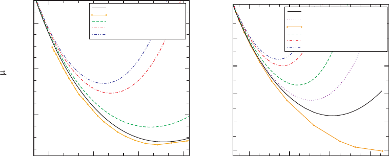
Figure 12.6 The binding energy E

vs. the orbital angular velocity 

orb

for corotational (left panel) and

nonspinning (right panel) equal-mass binaries. The solid lines mark the results of Cook and Pfeiffer (2004)and

Caudill et al. (2006), computed in the conformal thin-sandwich formalism with the equilibrium black hole

boundary conditions of Section 12.3.2 for corotating and exactly nonspinning black holes. The dotted line

labeled “LN” in the right panel was obtained similarly, except that the black holes are nonspinning to leading

order only. The solid dotted line labeled “CO: HKV-GGB” in the left panel marks the results of Grandcl

ement

et al. (2002), who use an approximate isometry boundary condition on the horizon. The solid dotted line labeled

“NS: IVP” marks the results from the Bowen–York effective potential approach, using the conformal imaging

technique (Cook, 1994). Finally, the dashed and dashed-dotted lines denote post-Newtonian “effective one-body”

results (Damour et al., 2002). [From Cook and Pfeiffer (2004)andCaudill et al. (2006).]

setting the magnitude of 

spin

equal to the magnitude of 

orb

in equation (12.107). Evalu-

ating the quasilocal spin (7.74) shows, however, that these black holes do not have exactly

vanishing spin as seen in the inertial frame, meaning that this sequence is not a truly non-

spinning sequence. We refer to this approach as the “leading-order approximation”. More

accurate results, representing exactly nonspinning black holes, can be obtained by iterating

over the parameter 

spin

until the quasilocal spin (7.74) does indeed vanish to a desired

accuracy.

Figure 12.5 includes curves of constant angular momentum; the extrema of these lines

mark quasicircular orbits as identiﬁed by the effective potential method. The solid line

connecting these extrema forms the corresponding quasiequilibrium inspiral sequence.

The dashed lines in Figure 12.5 mark the same sequence, but with circular orbits

identiﬁed by the mass criterion (12.108). The two approaches agree extremely well

up to very small binary separations, where the assumptions of quasiequilibrium break

down.

In Figure 12.6 we graph the binding energy of these inspiral sequences as a function of

the orbital angular speed 

orb

, which is a gauge invariant quantity. Also included in these

ﬁgures are results from other calculations. For the corotational sequence in the left panel

12.4 Quasiequilibrium sequences 425

of Figure 12.6 we include the numerical results of Grandcl

ement et al. (2002), who also

adopt the conformal thin-sandwich decomposition of Section 12.3, but, instead of using

the black hole equilibrium boundary conditions of Section 12.3.2, adopt an approximate

isometry condition.

It is reassuring that the numerical results differ only very little. For

the nonspinning sequence in the right panel we also include results for black holes that are

nonspinning to “leading-order” only, as well as the results from the Bowen–York effective

potential approach highlighted in Figure 12.3. Post-Newtonian results are also plotted for

comparison.

The turning points along the equilibrium binding energy curves in Figure 12.6 mark

their respective ISCOs, as discussed in Section 12.1. We tabulate the ISCO parameters in

Table 12.1 for corotational binaries and in Table 12.2 for nonspinning binaries. In these

tables we include numerical results, post-Newtonian results, as well as the results for a test

particle in circular orbit about a Schwarzschild black hole.

Exercise 12.13 Return to exercise 12.4 to reconsider a test particle of mass m

test

circular orbit about Schwarzschild black hole of mass M.

(a) Evaluate the results of that exercise to show that at the ISCO (areal radius r = 6M)

the test particle has an orbital angular velocity M

orb

= 1/6

3/2

≈ 0.0680, a bind-

ing energy E

test

≡−

√

8/9 − 1 ≈−0.0572 and an angular momentum

J/m

test

≡

= 2

√

3M ≈ 3.464M.

(b) Extrapolate the above results to estimate corresponding quantities for equal-mass

binary black holes in circular orbit with total irreducible mass m. To do this, interpret

the test mass m

test

as the reduced mass, m

test

→ µ = m/4, and the black hole mass

M as the total mass, M → m in the expressions found for part (a). Then derive the

values quoted in the last rows of Tables 12.1 and 12.2.

Actually, Tables 12.1 and 12.2 include two different sets of post-Newtonian results. The

ﬁrst set is a “standard” post-Newtonian expansion as described in Appendix E, except

that in the Appendix we focus on nonspinning objects only. For the nonspinning binaries

of Table 12.2, the ISCO parameters can be obtained directly from the minima of the

post-Newtonian expansion of the equilibrium binding energy (E.14). For the corotational

binaries of Table 12.1, however, certain spin contributions must be added to the binding

energy before the ISCO can be located.

The other set of post-Newtonian results is based

on an alternative “effective one-body” treatment,

which in some cases may accelerate

the convergence of the expansion.

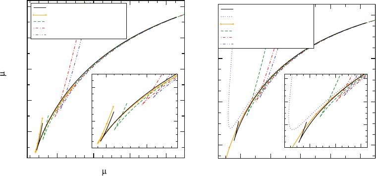
It is instructive to graph the equilibrium binding energy E

vs. the equilibrium angular

momentum J as in Figure 12.7. It is quite noticeable that most curves form a cusp.

These cusps are a consequence of equation (12.112), which implies that sequences of

constant irreducible mass must have simultaneous turning points in the ADM mass (hence

See the last paragraph in Section 12.3.1 and footnote .

See, e.g., Blanchet (2002, 2006).

Buonanno and Damour (1999); Damour et al. (2002).

426 Chapter 12 Binary black hole initial data

Table 12.1 The orbital angular velocity 

orb

, the equilibrium binding energy E

, and the equilibrium

angular momentum J at the ISCO of corotational, equal-mass, black hole binaries, as computed in

different calculations. The mass m is the total irreducible mass of the binary. Grandcl

ement et al. (2002)

and Caudill et al. (2006) adopt the conformal thin-sandwich decomposition; different choices in the

horizon boundary condition and the minimization procedure result in changes of at most a few percent.

Two sets of post-Newtonian results are included; one based on a “standard” post-Newtonian expansion

(Blanchet 2002) and another based on an “effective one-body” (EOB) approach (Damour et al. 2002).

[After Caudill et al. (2006).]

Corotational binaries m

orb

/mJ/m

Grandcl

ement et al. (2002) 0.103 −0.017 0.839

Caudill et al. (2006) 0.106 −0.0165 0.844

Blanchet (2002); 1PN – standard 0.5224 −0.0405 0.621

Blanchet (2002); 2PN – standard 0.0809 −0.0145 0.882

Blanchet (2002); 3PN – standard 0.0915 −0.0153 0.867

Damour et al. (2002); 1PN – EOB 0.0667 −0.0133 0.907

Damour et al. (2002); 2PN – EOB 0.0715 −0.0138 0.893

Damour et al. (2002); 3PN – EOB 0.0979 −0.0157 0.860

Test particle around Schwarzschild 0.068 −0.0143 0.866

Table 12.2 ISCO parameters for nonspinning, equal-mass black hole binaries for different calculations.

In addition to calculations referenced in Table 12.1, we also list the Bowen–York effective potential results

of Cook (1994)andBaumgarte (2000), who adopt the conformal imaging and puncture methods,

respectively, to treat the black hole singularities (see Section 12.2.2). [After Caudill et al. (2006).]

Nonspinning binaries m

orb

/mJ/m

Caudill et al. (2006) 0.122 −0.0194 0.779

Cook (1994) 0.166 −0.0225 0.744

Baumgarte (2000)0.18−0.023 0.74

Blanchet (2002); 1PN – standard 0.5224 −0.0405 0.621

Blanchet (2002); 2PN – standard 0.1371 −0.0199 0.779

Blanchet (2002); 3PN – standard 0.1287 −0.0193 0.786

Damour et al. (2002); 1PN – EOB 0.0692 −0.0144 0.866

Damour et al. (2002); 2PN – EOB 0.0732 −0.0150 0.852

Damour et al. (2002); 3PN – EOB 0.0882 −0.0167 0.820

Test particle around Schwarzschild 0.068 −0.0143 0.866

12.4 Quasiequilibrium sequences 427

3.6

4 4.4 4.8

J/ M

CO: MS -

CO: HKV - GGB

CO: EOB - 3PN

CO: EOB - 2PN

CO: EOB - 1PN

3.4

3.6

−0.06

−0.05

−0.02

−0.03

−0.04

−0.05

−0.06

−0.08

3.2

3.6

4.0 4.4 4.8

J/µM

/µ

NS: - d(αψ)/dr = (ψψ)/2r

d(αψ)/dr = (ψψ)/2r

LN: - d(ψψ)/dr = (

ψψ

)/2r

NS: IVP Conf.Imaging/Eff.Pot.

NS: EOB - 3P N

NS: EOB - 2P N

NS: EOB - 1P N

3 3.2 3.4

3.6

−0.08

−0.07

−0.06

−0.05

Figure 12.7 The equilibrium binding energy E

vs. the total equilibrium angular momentum J for the same

corotational (left panel) and nonspinning (right panel) binaries shown in Figure 12.6.[FromCook and Pfeiffer

(2004)andCaudill et al. (2006).]

the binding energy) and the angular momentum.

The nonspinning sequence for which

the black holes are nonspinning only to “leading-order”, however, does not feature such a

cusp – apparently this approximation is not sufﬁciently accurate at small binary separations

to produce a simultaneous turning point.

Several other aspects of the above ﬁgures and tables are noteworthy. The numerical

results of Grandcl

ement et al. (2002)andCook and Pfeiffer (2004) for corotational binaries

agree very closely, which is reassuring. Both post-Newtonian expansions seem to converge

to the conformal thin-sandwich data as the order of the expansion is increased. Since these

results are based on completely different approaches, this convergence presumably reﬂects

physical consistency in the solutions.

The ISCO parameters as obtained from the Bowen–York effective potential approach

differ signiﬁcantly from all other results. This discrepancy reconﬁrms our earlier concern

that the transverse-traceless decomposition does not provide direct means to construct

quasiequilibrium metrics, and suggests that the conformal thin-sandwich approach may be

the more promising approach. For binary separations outside the ISCO, however, Bowen–

York data agree reasonably well with other results (see, e.g., Figure 12.7). In fact, Bowen–

York puncture data have been used as initial data in many recent dynamical simulations

of binary black hole merger, partly because they are quite easy to construct, and partly

because they form a natural starting-point for the robust “moving puncture” evolution

technique that has been so widely adopted in many of these simulations (see Chapter 13).

Provided the binding energy is deﬁned as in equation (12.59); cf. footnote .

428 Chapter 12 Binary black hole initial data

Given the increasing speed and dynamic range of these simulations, it is possible to use

quasiequilibrium binaries of ever larger separation as initial data, whereby the distinctions

between different initial data sets are minimized.

One way of improving the above numerical results might be to abandon the assumption

of conformal ﬂatness ( ¯γ

= η

). We already know, for example, that this assumption

limits the maximum allowed spin of a rotating black hole constructed in the conformal

thin-sandwich approach (see the end of Section 3.3). By choosing the background metric

for binary black holes to be the superposition of two Kerr–Schild metrics, quasiequilibrium

binaries with quasilocal spin parmaters S

as large as 0.9998 have been constructed.

Most signiﬁcant, when evolved, these rapidly-spinning holes remain rapidly spinning even

after the initial relaxation, in contrast to the most rapidly spinning binaries constructed

with conformally-ﬂat metrics (either puncture or conformal thin-sandwich).

Another means of improvement might be to use post-Newtonian expressions for

the background data in the constraint equations.

A promising alternative could be the

“waveless approximation” described in Chapter 3.4. This approach allows a choice for the

time-derivative of the extrinsic curvature, whereby the evolution equation for the extrinsic

curvature turns into an equation for the conformally-related metric. Therefore, instead of

making an ad hoc choice for the latter, one can determine the conformal geometry that

results from some physical assumption. To date this approach has been implemented only

for binary neutron stars,

but it could be interesting to study binary black holes in the

future.

Lovelace et al. (2008); see also Liu et al. (2009).

Tichy et al. (2003).

Ury

u et al. (2006).

Binary black hole evolution

The dynamical simulation of the head-on collision of two black holes in axisymmetry

was an early success of numerical relativity (see Chapter 10.2). Based on this success one

might surmise that the subsequent simulation of the inspiral and merger of binary black

holes initially in circular orbit represented a straightforward generalization of the head-on

case. It turned out, however, that relaxing the assumption of axisymmetry to treat a binary

in circular orbit, and then tracking the resulting evolution, presented several nontrivial

challenges. As a consequence, dynamical simulations of these binaries were stalled for

many years until these challenges were ﬁnally overcome. Today, the inspiral and merger of

binary black holes is essentially a solved problem, constituting one of the major triumphs

of numerial relativity.

One obvious complication that arises in numerical simulations when moving from two

to three spatial dimensions is the burden of increased computational resources required

to cover the added dimension. Even though computers have become considerably faster

and can handle far more memory than the machines available when the ﬁrst head-on

black hole simulations were performed, the resources required to resolve inspiraling black

holes in the strong-ﬁeld, near-zone while simultaneously tracking and ultimately extracting

gravitational waves in the weak-ﬁeld, far-zone remain formidable. Different investigators

have adopted different approaches to address this problem of “dynamic range”, including

the use of ﬁxed or adaptive mesh reﬁnement or the construction of novel coordinate

systems that allocate gridpoints where they are most needed. In ﬁnite difference methods,

it is also possible to use higher-order differencing schemes in both space and time, like

fourth-order or higher, to increase the accuracy for a given number of grid points over the

more traditional second-order schemes featured in Chapter 6.2.

Another complication in going from two to three spatial dimensions arises from the form

of the evolution equations. In axisymmetry, it is not difﬁcult to formulate evolution schemes

that solve Einstein’s ﬁeld equations in a stable fashion when implemented numerically.

One such scheme is presented in Appendix F. At their core, the earliest formulations in

axisymmetry usually were based on the identiﬁcation of good “radiation variables” (see,

e.g., equations F. 5 and F. 6 ) and often employed one or more of the constraint equations

to solve for one or more of the metric variables in lieu of integrating the corresponding

evolution equation for the variable(s) (“constrained evolution”). In three spatial dimensions

429

430 Chapter 13 Binary black hole evolution

it has proven less obvious how to construct “radiation variables”,

and, as a result, it

is less clear how to arrive at a good choice for the form of the evolution equations.

Numerical implementations of the standard 3 + 1 or ADM equations as presented in

Chapter 2 develop instabilities, even for small perturbations of ﬂat space. As we discussed

in Chapter 11, several reformulations of the evolution equations have been developed that

do provide stable numerical implementations. These newer formulations, which include

the generalized harmonic system (Chapter 11.4) and the BSSN system (Chapter 11.5),

have led to dramatic breakthroughs in our ability to simulate the inspiral and merger of

binary black holes.

Finally, evolving black holes requires handling the singularities in their interiors, which,

if left unattended, could have dire consequences for a numerical simulation. For the head-on

collisions in axisymmetry it proved sufﬁcient to adopt singularity-avoiding coordinates to

deal with this issue (see Chapters 4 and 10.2), but for the longer-term evolutions required

for the simulations of binary black hole inspiral and merger, such coordinate systems

can lead to coordinate pathologies. One alternative approach that has proven successful

is the “excision” of the interior of the black hole in order to remove the singularity

from the computational domain. Another successful approach is the “moving puncture”

method, which is based on moving puncture gauge conditions. We will discuss both these

approaches in Section 13.1, after which we will summarize some successful simulations

of binary inspiral and merger in Section 13.2.

13.1 Handling the black hole singularity

Black hole interiors contain curvature singularities. If encountered during a numerical

simulation, these singularities can cause the calculation to terminate prematurely (i.e.,

“crash”). Special care therefore needs to be taken to avoid encountering such a singularity.

In the following we will discuss three approaches that have been used to avoid singularities:

singularity avoiding coordinates, black hole excision and the moving puncture method.

13.1.1 Singularity avoiding coordinates

To state the obvious, singularity avoiding coordinates are spacetime coordinates that avoid

singularities. A singularity avoiding time coordinate, for example, is one in which the

appearance of a spacetime singularity is postponed until t =∞. A popular example of

a such singularity avoiding slicing condition is maximal slicing (see Chapter 4.2 and,

in greater detail, Chapter 8.1). Black hole simulations using maximal slicing and other

singularity avoiding coordinate systems have been very successful in spherical symmetry

But see Bonazzola et al. (2004).

Unless, of course, the code is speciﬁcally designed to explore the properties of spacetime singularities; see, e.g., H

ubner,

(1996); Berger (2002).