Bhushan B. Handbook of Micro/Nano Tribology, Second Edition

Подождите немного. Документ загружается.

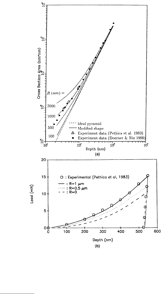
FIGURE 10.23 (a) Predicted projected contact area as a function of indentation depth curves for various tip radii

and measured data; (b) predicted load as a function of indentation depth curves for various tip radii and measured

data. (From Shih, C.W. et al., 1991, J. Mater. Res. 6, 2623–2628. With permission.)

We note that, for this example, tip shape calibration is necessary and the hardness is independent of

corrected depth. The hardness at any load used during indentation can be calculated, although generally

hardness only at peak load is calculated. For measurement of hardness at various loads, indentation

experiments at various peak loads corresponding to desired loads are generally carried out.

It should be pointed out that hardness measured using this deﬁnition may be different from that

obtained from the more conventional deﬁnition in which the area is determined by direct measurement

of the size of the residual hardness impression. The reason for the difference is that, in some materials,

a small portion of the contact area under load is not plastically deformed, and, as a result, the contact

area measured by observation of the residual hardness impression may be less than that at peak load.

However, for most materials, measurements using two techniques give similar results.

10.3.2 Modulus of Elasticity

Even though during loading a sample undergoes elastic–plastic deformation, the initial unloading is an

elastic event. Therefore, the Young’s modulus of elasticity or, simply, the elastic modulus of the specimen

can be inferred from the initial slope of the unloading curve (dW/dh) called stiffness (1/compliance) (at

the maximum load) (Figure 10.21). It should be noted that the contact stiffness is measured only at the

maximum load, and no restrictions are placed on the unloading data being linear during any portion of

the unloading.

If the area in contact remains constant during initial unloading, an approximate elastic solution is

obtained by analyzing a ﬂat punch whose area in contact with the specimen is equal to the projected

area of the actual punch. Based on the analysis of indentation of an elastic half space by a ﬂat cylindrical

punch by Sneddon (1965), Loubet et al. (1984) calculated the elastic deformation of an isotropic elastic

material with a ﬂat-ended cylindrical punch. They obtained an approximate relationship for compliance

(dh/dW) for the Vickers (square) indenter. King (1987) solved the problem of ﬂat-ended cylindrical,

quadrilateral (Vickers and Knoop), and triangular (Berkovich) punches indenting an elastic half-space.

He found that the compliance for the indenter is approximately independent of the shape (with a variation

of at most 3%) if the projected area is ﬁxed. Pharr et al. (1992) also veriﬁed that compliance of a paraboloid

of revolution of a smooth function is the same as that of a spherical or a ﬂat-ended cylindrical punch.

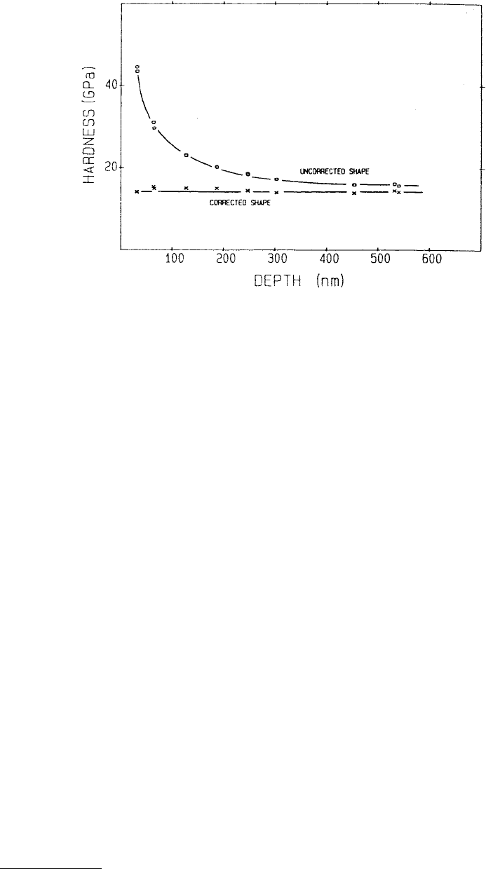
FIGURE 10.24 Hardness as a function of indentation depth for polished single-crystal silicon (111) calculated from

the area function with and without tip shape calibration. (From Doerner, M.F. and Nix, W.D., 1986, J. Mater. Res.

1, 601–609. With permission.)

The relationship for the compliance C (inverse of stiffness S) for an (Vickers, Knoop, and Berkovich)

indenter is given as

(10.6)

where

dW/dh is the slope of the unloading curve at the maximum load (Figure 10.21), E

, E

, and E

are the

reduced modulus and elastic moduli of the specimen and the indenter, and n

and n

are the Poisson’s

ratios of the specimen and indenter. C (or S) is the experimentally measured compliance (or stiffness)

at the maximum load during unloading, and A is the projected contact area at the maximum load.

The contact depth h

is related to the projected area of the indentation A for a real indenter by

Equation 10.4b. A plot of the measured compliance (dh/dW) vs. the reciprocal of the corrected indenta-

tion depth obtained from various indentation curves (one data point at maximum load for each curve)

should yield a straight line with slope proportional to 1/E

(Figure 10.25) (Doerner and Nix, 1986). E

can then be calculated, provided Poisson’s ratio with great precision is known to obtain a good value of

the modulus. For a diamond indenter, E

= 1140 GPa and n

= 0.07 are taken. In addition, the y-intercept

of the compliance vs. the reciprocal indentation depth plot should give any additional compliance that

is independent of the contact area. The compliance of the loading column is generally removed from the

load–displacement curve, whose measurement techniques will be described later.

We now discuss a preferred method to measure initial unloading stiffness (S). Doerner and Nix (1986)

measured S by ﬁtting a straight line about one third upper portion of the unloading curve. The problem

with this is that for nonlinear loading data, the measured stiffness depends on how much of the data is

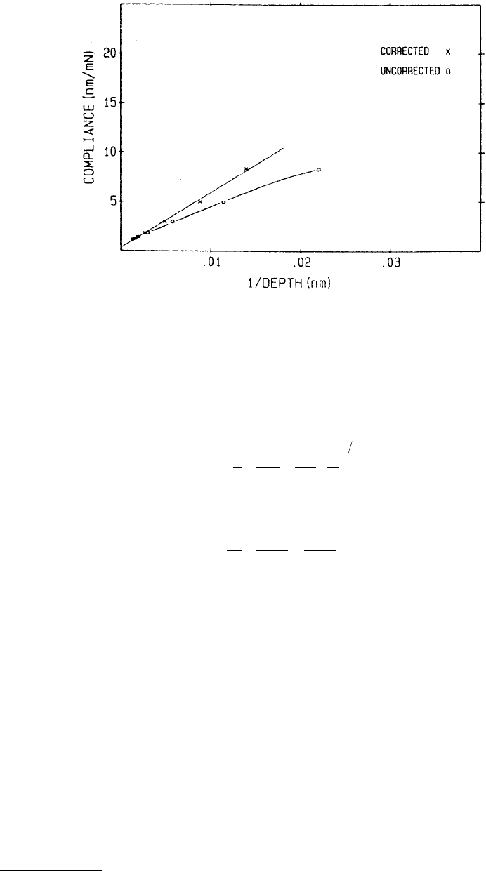
FIGURE 10.25 Compliance as a function of the inverse of indentation depth for tungsten with and without tip

shape calibration. A constant modulus with 1/depth would be indicated by the straight line. The slope of the corrected

curve is 480 GPa, which compares reasonably well to the known modulus of tungsten (420 GPa). The small y-intercept

of about 0.3 nm/mN is attributed to load-frame compliance, not removed. (From Doerner, M.F. and Nix, W.D.,

1986, J. Mater. Res. 1, 601–609. With permission.)

dW E A













EE E

−

−νν

used in the ﬁt. Oliver and Pharr (1992) proposed a new procedure. They found that the entire unloading

data are well described by a simple power law relation

(10.7)

where the constants B and m are determined by a least-square ﬁt. The initial unloading slope is then

found analytically, differentiating this expression and evaluating the derivative at the maximum load and

maximum depth. As we have pointed out earlier, unloading data used for the calculations should be

obtained after several loading/unloading cycles and with peak hold periods.

10.3.3 Determination of Load Frame Compliance

and Indenter Area Function

As stated earlier, measured displacements are the sum of the indentation depths in the specimen and the

displacements of suspending springs and the displacements associated with the measuring instruments,

referred to as load frame compliance. Therefore, to determine accurately the specimen depth, load frame

compliance must be known. This is especially important for large indentations made with high modulus

for which the load frame displacement can be a signiﬁcant fraction of the total displacement. The exact

shape of the diamond indenter tip needs to be measured because hardness and Young’s modulus of

elasticity depend on the contact areas derived from measured depths. The tip gets blunt (Figure 10.22)

and its shape signiﬁcantly affects the prediction of mechanical properties (Figures 10.23 through 10.25).

The method used in the past for determination of the area function has been to make a series of

indentations at various depths in materials in which the indenter displacement is predominantly plastic

and to measure the size of the indentations by direct imaging. Optical imaging cannot be used to measure

submicron-size impressions accurately. Because of the shallowness of the indent impressions, SEM results

in poor contrast.

A method consists of making two-stage carbon replicas of indentations in a soft material and imaging

them in the transmission electron microscope (TEM), was used initially by Pethica et al. (1983). Doerner

and Nix (1986) produced a series of indentations of varying size in annealed a–brass. Cellulose acetate

replicating tape was applied to the sample with a drop of acetone. Platinum with 20% palladium was

used as a shadowing agent. The indentations were oriented such that one side of the triangular perimeter

of each indentation was perpendicular to the shadowing direction. A shadowing angle of 19° was used.

Following shadowing, a carbon ﬁlm was evaporated onto the replica and the cellulose acetate removed

by dissolving in acetone. Doerner and Nix then imaged the prepared replicas at zero tilt in the transmitted

electron mode in the TEM. The areas of the indentations were measured and compared to the contact

depths as measured using the nanoindenter. An example of the calibration curve is shown in

Figure 10.23a. We can clearly see that use of the ideal geometry results in a large overestimate of the

hardness and modulus at small depths since the indenter tip is considerably more blunt than the ideal

pyramid. A calibration curve of the type shown in Figure 10.23a is used to determine the effective

indentation depth, h

eff

. The effective indentation depth is the depth needed for a pyramid of ideal

geometry to obtain a projected contact area equivalent to that of a real pyramid. Since the projected area

of ideal geometry of a Berkovich indenter is 24.5 h

, the effective indentation depth can be obtained

from the following equation:

(10.8)

where the area is obtained from the shape calibration and the true contact depth (Doerner and Nix,

1986). It is observed that ideal geometry underestimates the contact area which leads to overestimation

WBhh

=−

()

eff

Area

24.5













of hardness and modulus of elasticity especially at small indentation depths. For an example, see

Figures 10.24 and 10.25.

Oliver and Pharr (1992) proposed an easier method for determining area functions that requires no

imaging. Their method is based only on one assumption that Young’s modulus is independent of inden-

tation depth. They also proposed a method to determine load frame compliance. We ﬁrst describe the

methods for determining of load frame compliance followed by the method for area function. They

modeled the load frame and the specimen as two springs in series; thus,

(10.9)

where C, C

, and C

are the total measured compliance, specimen compliance, and load frame compliance,

respectively. From Equations 10.6 and 10.9, we get

(10.10)

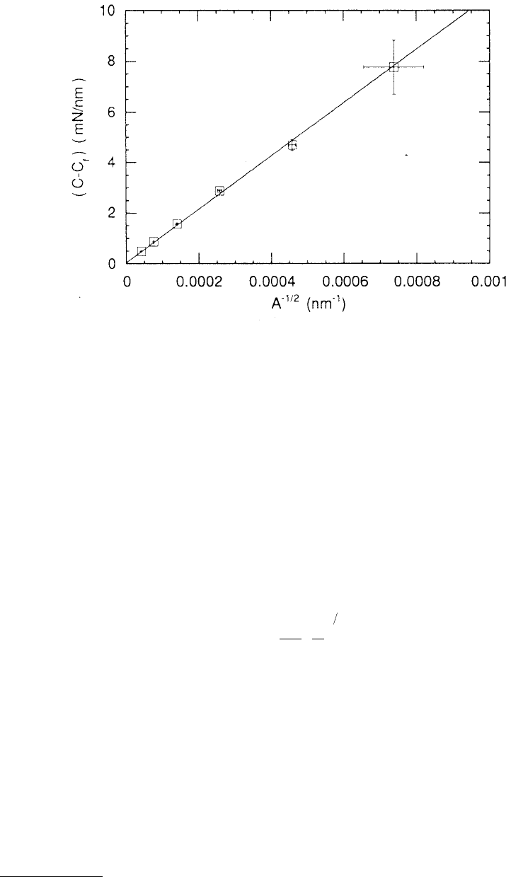
From Equation 10.10, we note that if the modulus of elasticity is constant, a plot of C as a function of A

1/2

is linear and the vertical intercept gives C

. It is obvious that most accurate values of C

are obtained

when the specimen compliance is small, i.e., for large indentations.

To determine the area function and the load frame compliance, Oliver and Pharr made relatively large

indentations in aluminum because of its low hardness. In addition, for the larger aluminum indentations

(typically 700 to 4000 nm deep), the area function for a perfect Berkovich indenter (Equation 10.4a) can

be used to provide a ﬁrst estimate of the contact. Values of C

and E

are thus obtained by plotting C as

a function of A

–1/2

for the large indentations, Figure 10.26.

Using the measured C

value, they calculated contact areas for indentations made at shallow depths

on the aluminum with measured E

and/or on a harder fused silica surface with published values of E

by rewriting Equation 10.10 as

FIGURE 10.26 Plot of (C – C

) as a function A

–1/2

for aluminum. The error bars are two standard deviations in

length. (From Oliver, W.C. and Pharr, G.M., 1992, J. Mater. Res. 7, 1564–1583. With permission.)

CC C













(10.11)

from which an initial guess at the area function was made by ﬁtting A as a function h

data to an eighth-

order polynomial

(10.12)

where C

through C

are constants. The ﬁrst term describes the perfect shape of the indenter; the others

describe deviations from the Berkovich geometry due to blunting of the tip. A convenient ﬁtting routine

is that contained in the Kaleidagraph software for Apple Macintosh computers. A weighted procedure

can be used to assure that data points with small and large magnitudes are of equal importance. An

iterative approach can be used to reﬁne the values of C

and E

further.

Now we describe the step-by-step procedure in detail, recommended by Oliver and Pharr (1992), for

determination of load frame compliance and indenter area function. It involves making a series of

indentations in two standard materials — aluminum and fused quartz — and relies on the facts that

both these materials are elastically isotropic, their moduli are well known, and their moduli are inde-

pendent of indentation depth. The ﬁrst step is to determine precisely the load frame compliance. This

is best accomplished by indenting a well-annealed, high-purity aluminum which is chosen because it is

readily available, has a low hardness, and is nearly elastically isotropic. Some care must be exercised in

preparing the aluminum to assure that its surface is smooth and unaffected by work hardening. A series

of indentations are made in the aluminum using the ﬁrst six peak loads, and loading rates shown in

Table 10.3. Typically indentation depths range from 700 to 4000 nm. The load time history recommended

by Oliver and Pharr is as follows: (1) approach and contact surface, (2) load to peak load, (3) unload to

90% of peak load and hold for 100 s, (4) reload to peak load and hold for 10 s, and (5) unload completely

at half the rate shown in Table 10.3. The lower hold is used to establish thermal drift and the upper hold

to minimize time-dependent plastic effects. The ﬁnal unloading data are used to determine the unloading

compliances using the power law ﬁtting procedure described earlier. The load frame compliance is

TABLE 10.3 Peak Loads and Loading/Unloading Rates Used in the Load Frame Compliance

and Area Function Calibration Procedures

Indentation

Numbers Peak Load (mN) Loading/Unloading Rate (µN/s) Nanoindenter Load Range

For Load-Frame Compliance

1–10 120 12000 High

11–20 60 6000 High

21–30 30 3000 High

31–40 15 1500 High

41–50 7.5 750 High

51–60 3 300 High

For Area Function

61–70 20 2000 Low

71–80 10 1000 Low

81–90 3 300 Low

91–100 1 100 Low

101–110 0.3 30 Low

111–120 0.1 10 Low

From Oliver, W.C. and Pharr, G.M., 1992, J. Mater. Res. 7, 1564–1583. With permission.

−

()

A h Ch Ch Ch Ch

ccc c c

=++++…+24 5

1 128

determined from the aluminum data by plotting the measured compliance as a function of area calculated,

assuming the ideal Berkovich indenter. Calculated E

is checked with known elastic constants for alumi-

num, E = 70.4 GPa and n = 0.347. The values of the elastic constants we use for the diamond indenter

are E

= 1141 GPa and n

= 0.07.

The problem with using aluminum to extend the area function to small depths is that because of its

low hardness, small indentations in aluminum require very small loads, and a limit is set by the force

resolution of the indentation system. This problem can be avoided by making the small indentations in

fused quartz, a much harder, isotropic material available in optically ﬁnished plate form. The standard

procedure that Oliver and Pharr recommend for determining the area function involves making a series

of indentations in fused quartz using the second set of six peak loads shown in Table 10.3. For the loads

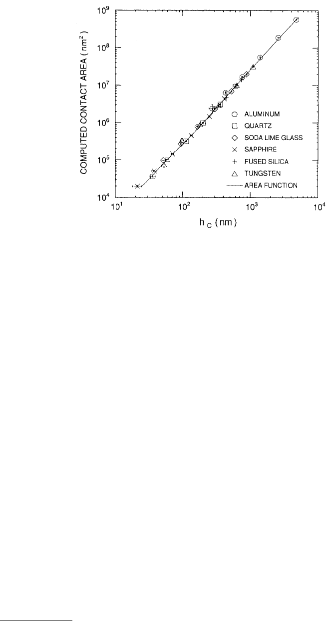
outlined in Table 10.3, the minimum contact depth is about 15 nm and the maximum about 4700 nm.

(Typically measurements are made at depths ranging from about 15 to 700 nm. Above 700 nm of depth,

indenter can be assumed to have a perfect shape.) The contact areas and contact depths are then

determined using Equation 10.12 and h

in conjunction with the reduced modulus computed from the

elastic constant for fused quartz, E = 72 GPa and n = 0.170. The machine compliance is known from the

aluminum analysis. The area function is only good for the depth range used in the calculations. Typical

data of contact areas as a function of contact depths for six materials is shown in Figure 10.27.

10.3.4 Hardness/Modulus

Parameter

Calculations of hardness and modulus described so far require the calculations of the indent projected area

from the indentation depth, which are based on the assumption that the test surface be smooth to dimen-

sions much smaller than the projected area. Therefore, data obtained from rough samples show considerable

scatter. Joslin and Oliver (1990) developed an alternative method for data analysis without requiring the

calculations of the projected area of the indent. This method provides measurement of a parameter hard-

ness/modulus

, which provides a measure of the resistance of the material to plastic penetration.

FIGURE 10.27 The computed contact areas as a function of contact depths for six materials. The error bars are

two standard deviations in length. (From Oliver, W.C. and Pharr, G.M., 1992, J. Mater. Res. 7, 1564–1583. With

permission.)

They showed that for several types of rigid punches (cone, ﬂat punch, parabola of revolution, and

sphere) as long as there is a single contact between the indenter and the specimen,

(10.13)

where S is the stiffness obtained from the unloading curve. E

is related to E

by a factor of 1 – n

for

materials with moduli signiﬁcantly less than diamond (Equation 10.6). H/E

parameter represents a

materials resistance to plastic penetration. We clearly see that calculation of projected area and knowledge

of area function are not required. However, this method does not give the hardness and modulus values

separately.

10.3.5 Continuous Stiffness Measurement

Oliver and Pethica (1989) and Pethica and Oliver (1989) developed a dynamic technique for continuous

measurement of sample stiffness during indentation without the need for discrete unloading cycles, and

with a time constant that is at least three orders of magnitude smaller than the time constant of the more

conventional method of determining stiffness from the slope of an unloading curve. Furthermore, the

measurements can be made at exceedingly small penetration depths. (Also see Wu, 1993.) Thus, their

method is ideal for determining the stiffness and, hence, the elastic modulus and hardness of ﬁlms a few

tens of a nanometers thick. Furthermore, its small time constant makes it especially useful in measuring

the properties of some polymeric materials.

Measurement of continuous stiffness is accomplished by the superposition of a very small AC current

of a known relatively high frequency (typically 69.3 Hz) on the loading coil of the indenter. This current,

which is much smaller than the DC current that determines the nominal load on the indenter, causes

the indenter to vibrate with a frequency related to the stiffness of the sample and to the indenter contact

area. A comparison of the phase and amplitude of the indenter vibrations (determined with a lock-in

ampliﬁer) with the phase and amplitude of the imposed AC signal allows the stiffness to be calculated

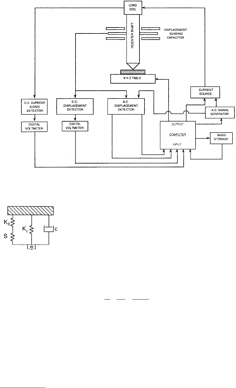
either in terms of amplitude or phase. Figure 10.28 is a schematic wiring diagram illustrating the oper-

ation of continuous-stiffness option. The displacement as small as 0.001 nm can be measured using

frequency-speciﬁc ampliﬁcation. The time constant of about 0.33 s provides a good combination of low

noise and dynamic response.

To calculate the stiffness of the contact zone, the dynamic response of the indentation system has to

be determined. The relevant components are the mass m of the indenter, the spring constant K

of the

leaf springs that support the indenter, the stiffness of the indenter frame K

, and the damping constant

C due to the air in the gaps of the capacitor plate displacement-sensing system. These combine with the

stiffness of the contact zone (sample stiffness) S, as shown schematically in Figure 10.29 to produce the

overall response. If the imposed driving force is F = F

exp(iwt) and the displacement response of the

indenter is a = a

exp(iwt + f), the ratio of amplitudes of the imposed force and the displacement response

is given by (Pethica and Oliver, 1989)

(10.14)

and the phase angle, f, between the driving force and the response is

(10.15)

HE WS

4=π

()

cKm

22 2

=+−

()













ωω

tan φω ω=−

()

cKm

where w is the frequency of the imposed force, c is the damping constant for the central plate of the

displacement capacitor (damping due to the air in the capacitor gaps), and m is the mass of the indenter

assembly. K, the combined spring constant for the system, is given by

(10.16)

With the exception of S, all the terms in Equations 10.14 and 10.15 can be measured independently.

Thus, the displacement signal resulting from the imposition of the DC current is measured with a phase-

sensitive detector (lock-in ampliﬁer), which yields both the amplitude and phase angle of the displace-

ment signal. The AC input to the force coil is generated with a standard AC signal generator, and any

frequency between about 10 and 150 Hz may be selected. The stiffness S can be determined either from

phase angle f or from amplitude a

of response. Pethica and Oliver (1989) pointed out that f will be most

sensitive to small values of S and a

will be best for larger values of S.

FIGURE 10.28 Schematic wiring diagram of the nanoindenter with the continuous stiffness measurement option.

(Courtesy of Nano Instruments, Knoxville, TN.)

FIGURE 10.29 Components of the dynamic model of the indentation system.

(From Pethica, J.B. and Oliver, W.C., 1989, in Thin Films: Stresses and Mechanical

Properties, J.C. Bravman et al., eds., Vol. 130, pp. 13–23, Materials Research Society,

Pittsburgh. With permission.)

11 1

KK KS

10.3.6 Modulus of Elasticity by Cantilever Deﬂection Measurement

The submicron indentation of thin ﬁlms on substrates can lead to quick and accurate measurement of

hardness, but the large pressures under the indenter may alter the structure of thin ﬁlms being tested.

For submicron (<200 nm) ﬁlms, the inﬂuence of the substrate must be considered. With wafer curvature

techniques, the average stress and strain in a ﬁlm can be measured, but the range of stresses is limited

by the thermal expansion and/or growth mismatch of the substrate and the ﬁlm. Thus, for a given ﬁlm

and substrate, one cannot dictate the stress to be applied to the ﬁlm. In an effort to avoid some of these

difﬁculties, Weihs et al. (1988) developed a new technique based on the deﬂection of free-standing

cantilever microbeams. Brieﬂy, the technique involves the fabrication of the beams using silicon micro-

machining techniques and the deﬂection of the beams using a nanoindenter. The nanoindenter mechan-

ically bends the beams while continuously monitoring the loading and the deﬂection of the beams. Using

this technique, both elastic modulus and yield strength can be studied.

Weihs et al. measured properties of free-standing beams of SiO

, LTO, and gold coatings used in VLSI

fabrication cut into small sections (15 ¥ 15 mm). These beams were mounted on aluminum blocks with

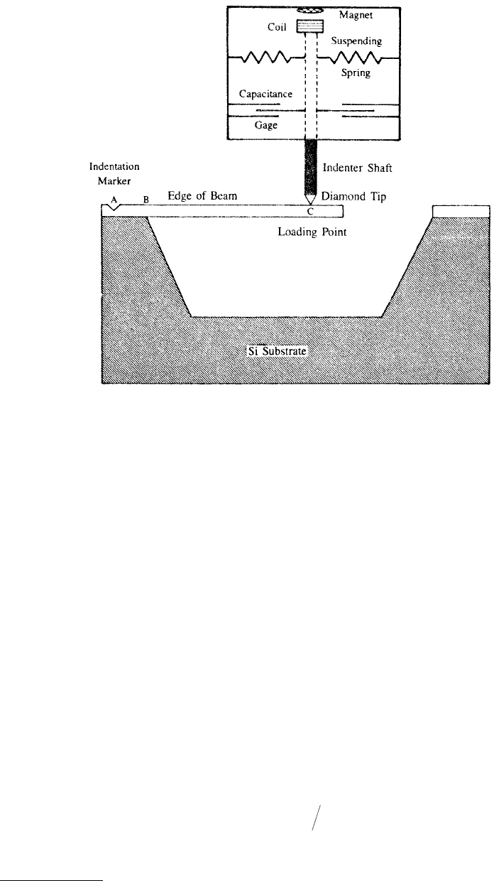
crystal bond wax, Figure 10.30. The microbeams were deﬂected at velocities ranging from 3 to 60 nm/s.

Typical dimensions of the beam free to deﬂect were 40-µm length, 20-µm width, and 1-µm thickness.

The modulus of elasticity is calculated from the following equation valid for small deﬂection of a thin ﬁlm:

(10.17)

FIGURE 10.30 Schematic of a cantilever microbeam deﬂected by nanoindenter loading mechanism for measure-

ment of modulus of elasticity and yield strength of microbeam material. (From Weihs, T.P. et al., 1988, J. Mater. Res.

3, 931–942. With permission.)

h W bt E=−

()()

323

l ν