Canete J.F. System Engineering and Automation: An Interactive Educational Approach
Подождите немного. Документ загружается.

38 2 System Modeling
(a)
(b)
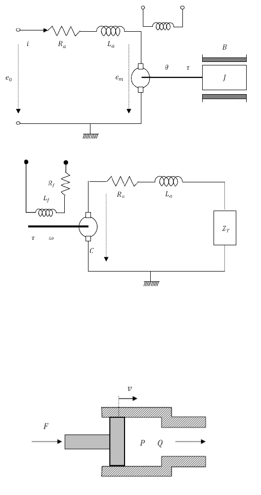
Fig. 2.31 Schematic of the DC motor (a) and DC generator (b) devices.
On the other hand, the hydromechanical translational converter represents an
ideal hydraulic piston, whose primary use is as a mechanical drive (fig. 2.32).
Fig. 2.32 Schematic of the hydraulic piston device.
2.7 Hybrid Systems 39
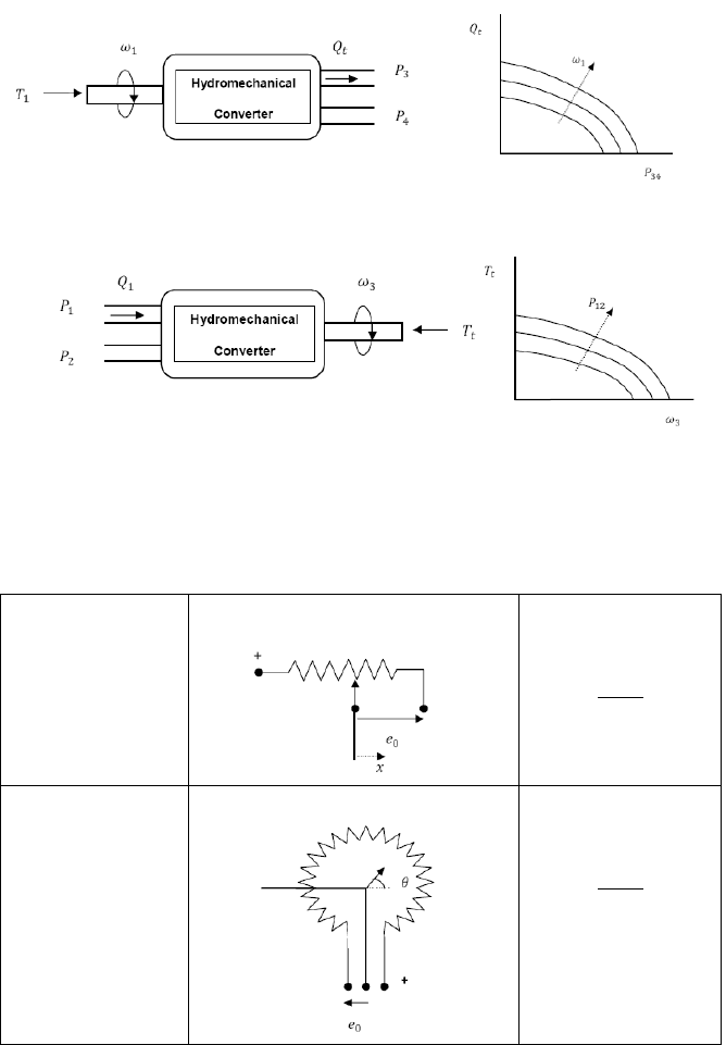
Meanwhile, the hydromechanical rotational converter represents both an ideal
centrifugal pump and an ideal hydraulic turbine, whose primary use is in hydraulic
drive systems (fig. 2.33).
(a)
(b)
Fig. 2.33 Schematic of the centrifugal pump (a) and hydraulic turbine (b) devices.
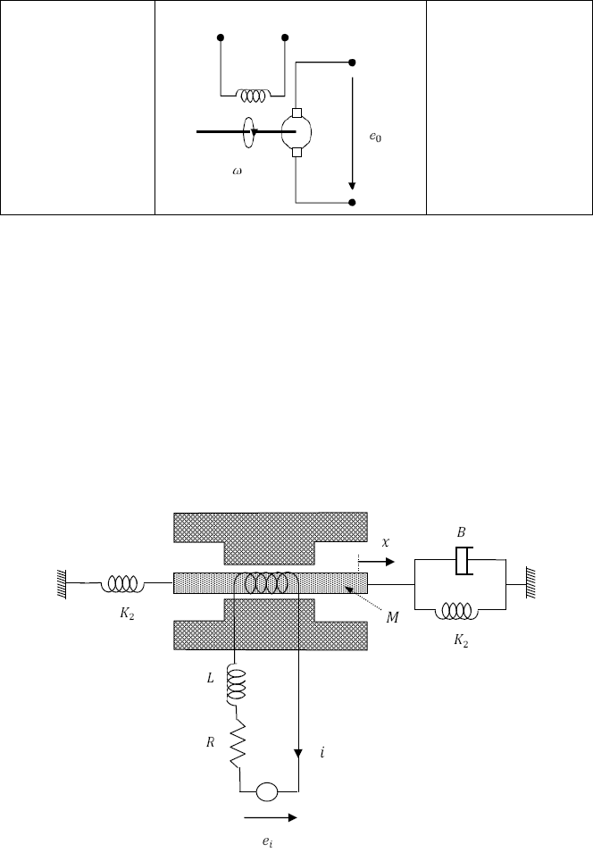
Table 2.10 Some signal converting transducers with corresponding dynamic equations
Translational
Potentiometer
Rotational
Potentiometer
40 2 System Modeling
Table 2.10 (continued)
Tachometer
Besides this, also to be included are the signal converting transducers,
characterized for being energy converters that have a negligible load, such as
potentiometers, and tachometers among others. In table 2.10 these converting
transducers with its corresponding icons and dynamic equations are described.
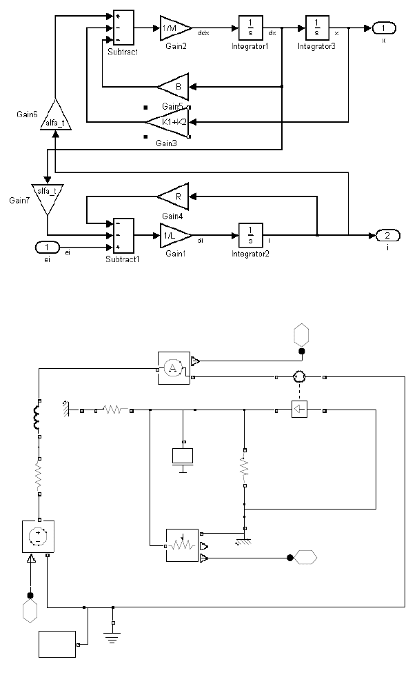
Example 2.7
Derive the dynamic equations corresponding to the electromechanic circuit shown
in fig. 2.34, with e
i
(t) considered as input and x(t) and i(t) considered as output of
the system respectively, also drawing the corresponding SIMULINK and
SIMSCAPE modeling diagrams.
Fig. 2.34 Hybrid electromechanic system for example 2.7.
2.7 Hybrid Systems 41
Fig. 2.35 SIMULINK diagram corresponding to example 2.7
Fig. 2.36 SIMSCAPE diagram corresponding to example 2.7
i3
x
2
ei 1
x
R
C
V
P
k2
R
C
i
+
I
-
ei
Solver
Co nfiguration
f(x)=0
R
+
-
M
L
+
-
K1
R
C
Ground
Converter
+
-
R
C

42 2 System Modeling
Solution
In fig. 2.35 and fig. 2.36 the corresponding modeling diagram developed by using
both the SIMULINK and SIMSCAPE environments are shown.
Chapter 3
System Description
This chapter deals with the description of continuous-time systems, in particular,
the external and internal description of linear and time invariant (LTI) type, and
introduces the linearization technique employed for approximating nonlinear
system behavior.
The Laplace transform method to find the analytical response of LTI systems to
different input signals is also described. We also derive the transfer function as a
mean to represent LTI systems in the Laplace domain, both for univariable and
multivariable systems. The state space approach and its relation to the transfer
function are also treated.
Finally, we describe the techniques to obtain block diagrams starting from
dynamical equations for LTI systems, and the block reduction techniques for
obtaining a unique transfer function representing the system behavior.
Accompanying the subject matter, some applications are illustrated in MATLAB
code to improve the concepts described.
3.1 Continuous Time Systems
A continuous-time system is one for which the inputs, state variables and outputs
are defined over some continuous range of time, and its behavior is described by
differential equations.
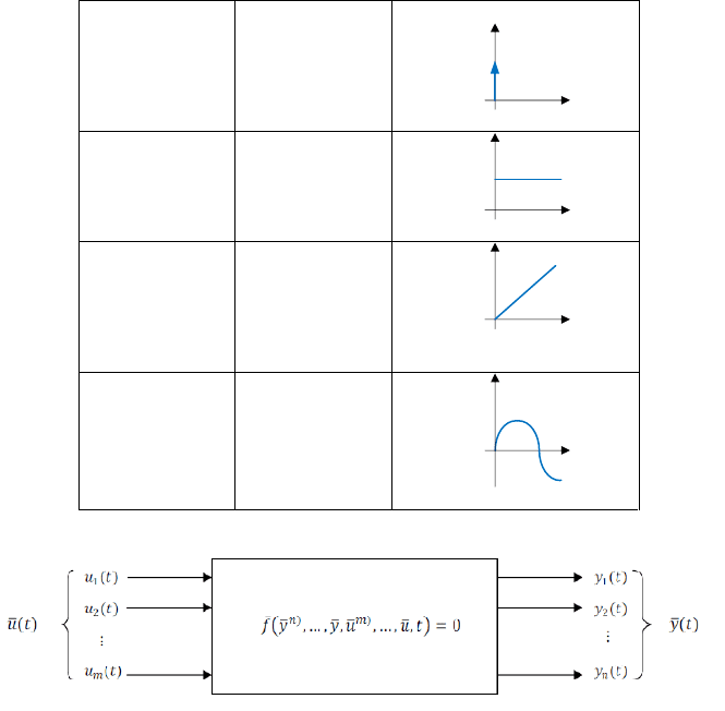
Some of the input signals are used as test signals both to analyze the system
behavior or to design control systems. These inputs are the impulse, step, ramp, or
sinusoidal as is shown in table 3.1.
In general, a continuous system with r inputs and s outputs (fig. 3.1) can be
described by s independent input-output differential equations
,…,
,
,
…,
,…,
,
,
,…,
,
,…,
,…,
,
,0
,…,
,
,
…,
,…,
,
,
,…,
,
,…,
,…,
,
,0
,…,
,
,
…,
,…,
,
,
,…,
,
,…,
,…,
,
,0
(3.1)
where for causal behavior, with
,1,…., non-linear in general. The
parameter n is denoted as the system order, and plays a fundamental role for the
system behavior.
44 3 System Description
Table 3.1 Some test input signals used for system analysis
Impulse
Step
Ramp
Senoidal
sin
Fig. 3.1 Continuous multi-input, multi-output system.
If the system is single-input and single-output, the continuous dynamic
differential equation is given by
,…,
,
,
…,
,,0
(3.2)
where for causal behavior, with f non-linear in general.
Analytical methods for exact solving (3.1) given the input signals and an
appropriate set of initial conditions are practical only for low order and system
dynamics described rather by (3.2). Nevertheless, the application of numerical
methods will enable to deal with high order and multi-input, multi-output to obtain
approximate solutions.
3.2 Linear and Invariant Time Systems 45
Let us particularize the analysis for a single input single output system, with f
described by a linear combination of both input and output signals together with
its derivatives, assuming also the system is stationary, and no direct dependence
with time t is made explicit.
3.2 Linear and Invariant Time Systems
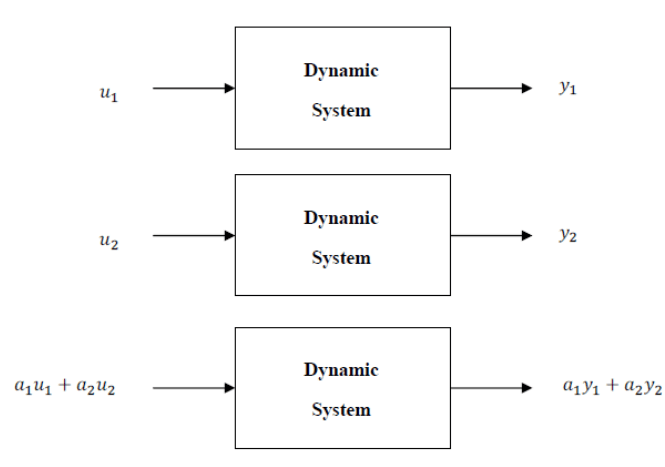
It is said that a system is linear when it fulfills the principle of superposition,
which states that the system's response to a set of simultaneous inputs can be
decomposed into the sum of individual responses (fig. 3.2). On the contrary,
nonlinear systems are those which superposition does not hold.
Fig. 3.2 The application of the principle of superposition
A continuous-time system defined by differential equations is said to be linear
if it can be expressed as a linear combination of derivatives of the output and input
in the form
(3.3)
where the parameters
,1… and
,1 … are constants or
functions of time t. In the event that these parameters do not depend explicitly on
the time t, the system is said to be also time-invariant, and if it is not the case, the
system is said to be nonlinear.
46 3 System Description
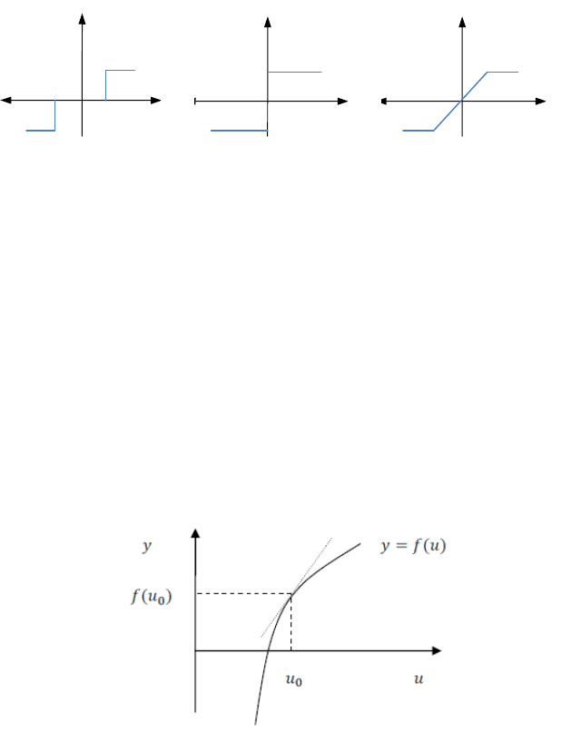
Nearly all systems are inherently nonlinear in nature, since most of the
relationships in physics are nonlinear. Moreover, most of the linear systems are a
special case of nonlinear systems in limited ranges of operation. Besides this, the
nonlinear nature of the physical elements constituting the system may be an
essential feature of the system, causing the overall system behavior to be nonlinear
as with the dead zone, relay, saturation, etc. characteristics (fig. 3.3).
Fig. 3.3 Some examples of nonlinear relationships
3.3 Systems Linearization
The objective of the linearization technique is to derive a linear approximate
system whose response will agree closely with that of the original nonlinear
system which it comes from.
In order to apply linearization method, we use the disturbance method, which
consists in considering small variations around a nominal operating point, making
into the non-linear relationship , the following substitutions:
1. The independent variable u is replaced by
,
being the
operating point of u, and the disturbance applied on u.
2. The dependent variable or curve representing the non-linearity
is replaced by its tangent at the nominal operating point u
(fig. 3.4).
Fig. 3.4 Linearization of at operation point

3.3 Systems Linearization 47
Approximating
by the Taylor’s expansion we have
1
2!
(3.4)
Approaching the nonlinear relation by its first derivative (tangent of the curve) it
follows that
(3.5)
which represents the substitution to be made on the dependent variable y whenever
.
By extending this method to a multivariable nonlinear relationship
,
,…,
in general, we have
,…,
,…,
(3.6)
where
,
,…,
the nominal operating point, where the partial
derivatives of f w.r.t. to
are evaluated at
.
In case nonlinear system relationship is given by a set of differential equations,
the disturbance method in implicit form will be applied to
,…,
,,
,…,
,0
(3.7)
Therefore, following the same approach used in (3.6), we have
,…,
,,
,…,
,
,…,
,
,
,…,
,
(3.8)
The nominal operating point
,
around which we will make the
linearization, is necessarily the solution of the differential equation describing the
system dynamics, and is derived from equation (3.7), making zero, the derivatives
of the implicit differential equation at
in