Canete J.F. System Engineering and Automation: An Interactive Educational Approach
Подождите немного. Документ загружается.

48 3 System Description
,…,
,
,
,…,
,
0
(3.9)
In this way, the second term on the right hand side of (3.8) is the differential
equation linearized around the nominal operating point
,
, that is
approximated by
0
(3.10)
where the partial derivatives of F w.r.t. to each independent variables of (3.7) are
evaluated at
, and whose validity is restricted to a small region
around
.
Example 3.1
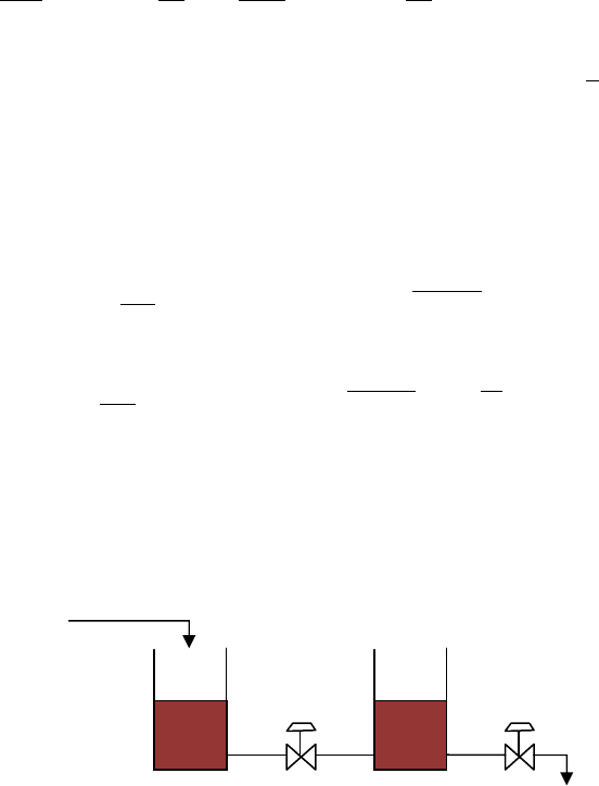
The diagram of (fig. 3.5) represents a two tank in series system, whose dynamics
is given by the set of nonlinear differential equations
,
,
,
,
where h
1
, h
2
, and q
e
respectively are the height of tank 1, tank 2 and input flow to
tank 1, while the rest of parameters A
1
, A
2
, K
1,
and K
2
stand for the tank areas and
the discharge coefficient.
Obtain the linearized system around the operation point
.
Fig. 3.5 Linearization of a two tank system.
h
1
h
2
q
e

3.3 Systems Linearization 49
Solution
In first place we must express the system equations in implicit form, so as to
derive the linearized approximated system, calculating afterwards the operation
point
,
,
.
,
,
,
,
0
,
,
,
,
0
Making zero the derivatives in both equations we have a system equation for
solving h
10
and h
20
as a function of q
e0
, so we have
0
Now, the partial derivatives of F
1
and F
2
w.r.t. to the dependent variables at
,
,
are calculated, that is,
2
2
2
0
0
2
2
1
0
Thus, defining the incremental variables as
,
, and
, we have the linearized equation set
2
2
50 3 System Description
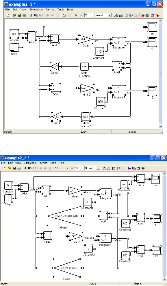
Fig. 3.6 SIMULINK diagram corresponding to the nonlinear two tank system.
Fig. 3.7 SIMULINK diagram corresponding to the linearized two tank system.
3.4 Laplace Transfor
m
51
In fig. 3.6 we show the SIMULINK diagrams corresponding to the nonlinear
two tank system and its linearized approximation (fig. 3.7), together with their
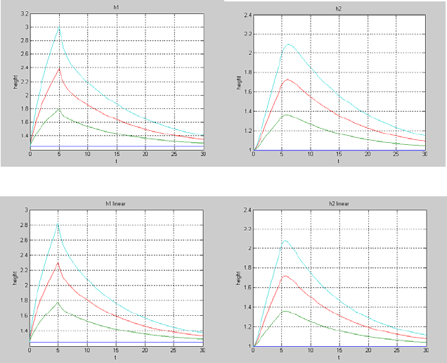
responses to pulse step input with increasing amplitude. For this experience, we
have selected an operating point
,
,
1.25,1.0,1.0 after
solving the linearization point equations for q
e0
= 1.0., with A
1
= 2.0, A
2
= 3.0, K
1
=
2.0 and K
2
= 1.0, using an incremental amplitude for q
e
from 1.0 to 2.0.
We can observe that as long as the incremental input amplitude
remains
closer to the operation point, no significant differences are observed between the
nonlinear and linearized responses to pulse changes (fig. 3.8).
(a)
(b)
Fig. 3.8 Response to incremental pulse changes in q
e
corresponding both to the nonlinear
(a) and to the linearized (b) two tank system.
3.4 Laplace Transform
The technique of Laplace transform is used to solve the linear differential
equations with constant coefficients expressed in the time domain which define
the linear system behavior, thus transforming them into linear algebraic equations
expressed in a complex domain.

52 3 System Description
3.4.1 Direct Laplace Transform
The Laplace transform of is represented symbolically as
and is
defined as
(3.11)
where is a complex variable.
Applying equation (3.11) it is possible to derive a pair
for each
function, so that it is possible to derive a complete table for the most
representative input and output signals appearing in dynamic continuous system.
Example 3.2
Derive the Laplace transform of the impulse, step and ramp signals.
Solution
1.
1, therefore
1
2.
, therefore
3.
, applying the integration by
parts,
, therefore
Nevertheless, in order to find the transform pairs for complex signals and to solve
for the responses of dynamic linear systems given by (3.3), we illustrate some
useful properties of the Laplace transform:
a) Linearity
(3.12)
b) Damping
(3.13)
c) Displacement in time
(3.14)

3.4 Laplace Transfor
m
53
Table 3.2 Laplace transforms table
Function f(t) Laplace Transform F(s)
1
1
1
1
1
1
!
!
d) Differentiation
0
0
0
(3.15)
being
0
,
0
,…,
0 the set of initial conditions for .

54 3 System Description
e) Integration
1
(3.16)
f) Multiplication by time
1
(3.17)
g) Multiplication
(3.18)
h) Final Value
∞
lim
lim
(3.19)
Then, by combining the Laplace transform of simple signals with the properties
described above, it is possible to build a table of Laplace transforms to derive the
transform of common functions which appear frequently when the system
response is demanded (table 3.2)
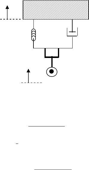
Example 3.3
Derive the step response corresponding to the mechanical system shown in
fig. 3.9 whose dynamic equation is given by
for values of M = 1, D = 6 and K = 9, starting from initial conditions
0
0 and
0
0.
Solution
Applying the Laplace transform properties we get
3.4 Laplace Transfor
m
55
Fig. 3.9 Diagram of the mechanical system for example 3.3.
so that the system response is given by
1
In case of step input
, so that the system response Y(s) particularized for
M, D, and K is given by
1
69
3.4.2 Inverse Laplace Transform
Once we get the Laplace transform of the response of a continuous linear and
invariant system as described by (3.3), it is necessary to derive the temporal
response by applying the inverse Laplace transform, which enables to restore
the time response format.
The inverse Laplace transform of is represented symbolically as
and is defined as the integral in the complex domain
,0
(3.20)
where is a selected value to the right of all the singularities of in the s
plane.
In practice, this relation is seldom used, as the Laplace transform is given
as a proper rational function in s
K
D
M
y(t)
F(t)

56 3 System Description
(3.21)
with , such that this complex Laplace transform will be broken down into
simpler ones that are listed in table 3.2 along with their corresponding time
responses.
For this reason, we apply the partial fraction expansion method to obtain such
simpler transforms, by calculating in first place the roots of , making
0
…
(3.22)
for
,1… distinct roots, with multiplicity of
and complex in general.
By factoring the rational function into its partial fraction expansion, we
have in case of single roots and distinct
(3.23)
where the constants
or residuals of
are given by
lim
1…
(3.24)
while in case of multiple roots we decompose in
(3.25)
where the residuals
of
are defined by
1
!
lim
1…, 1,…
(3.26)
Once the residuals are determined, we proceed to calculate the inverse Laplace
transforms of each individual fraction of (3.25) by identifying the corresponding
time function associated in table 3.2, and then use the superposition relation to
obtain the desired function
.

3.4 Laplace Transfor
m
57
In case of complex conjugate roots, it is necessary to group the corresponding
partial fractions prior to identifying the inverse transform in table 3.2. Assuming
that the complex roots are located in
and
, the
corresponding partial fractions are given by
Applying (3.24) we obtain the residuals
lim
lim
where
and
a pair if complex conjugate residuals.
Grouping the two partial fractions we have
with
2
and
2
, so it is now possible to calculate the inverse
Laplace transforms of each individual fraction by identifying the corresponding
time function associated in table 3.2.
Example 3.4
Obtain the step response y
t
corresponding to fig. 3.9 starting from the preceding
value of , using the MATLAB commands necessary to derive the residues
and to plot the time response.
Solution
Starting from of (3.31), we calculate the roots of the denominator
690
by applying the MATLAB code
>> den= [1 6 9 0];
>> roots(den);
ans =
0
-3.0000
-3.0000