Devore J.L., Berk K.N. Modern Mathematical Statistics with Applications

Подождите немного. Документ загружается.

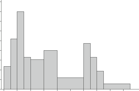
This histogram has three rather distinct peaks: the first corresponding to

lightweight players like defensive backs and wide receivers, the second to “medium

weight” players like linebackers, and the third to the heavyweights who play

offensive or defensive line positions.

■

When class widths are unequal, not using a density scale will give a picture

with distorted areas. For equal-class widths, the divisor is the same in each density

calculation, and the extra arithmetic simply results in a rescaling of the vertical axis

(i.e., the histogram using relative frequency and the one using density will have

exactly the same appearance). A density histogram does have one interesting

property. Multiplying both sides of the formula for density by the class width gives

relative frequency ¼ðclass widthÞðdensityÞ¼ðrectangle widthÞðrectangle heightÞ

¼ rectangle area

That is, the area of each rectangle is the relative frequency of the corresponding

class. Furthermore, because the sum of relative frequencies must be 1.0 (except for

roundoff), the total area of all rectangles in a density histogram is l. It is always

possible to draw a histogram so that the area equals the relative frequency (this is true

also for a histogram of counting data)—just use the density scale. This property will

play an important role in creating models for distributions in Chapter 4.

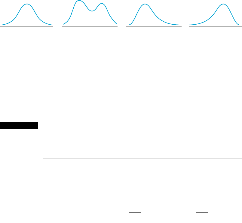
Histogram Shapes

Histograms come in a variety of shapes. A unimodal histogram is one that rises to a

single peak and then declines. A bimodal histogram has two different peaks.

Bimodality can occur when the data set consists of observations on two quite

different kinds of individuals or objects. For example, consider a large data set

0.018

0.016

0.014

0.012

0.010

0.008

0.006

0.004

0.002

0.000

180 200 220 240 260 280 300 320 340 360

Density

Weight

Figure 1.9 A MINITAB density histogram for the weight data of Example 1.9

CHAPTER 1 Overview and Descriptive Statistics

consisting of driving times for automobiles traveling between San Luis Obispo and

Monterey in California (exclusive of stopping time for sightseeing, eating, etc.).

This histogram would show two peaks, one for those cars that took the inland route

(roughly 2.5 h) and another for those cars traveling up the coast (3.5–4 h). However,

bimodality does not automatically follow in such situations. Only if the two

separate histograms are “far apart” relative to their spreads will bimodality occur

in the histogr am of combined data. Thus a large data set consisting of heights of

college students should not result in a bimodal histogram because the typical male

height of about 69 in. is not far enough above the typical female height of about

64–65 in. A histogram with more than two peaks is said to be multimodal.

A histogram is symmetric if the left half is a mirror image of the right half.

A unimodal histogram is positively skewed if the right or upper tail is stretched out

compared with the left or lower tail and negatively skewed if the stretching is to the

left. Figure 1.10 shows “smoothed” histograms, obtained by superimposing a

smooth curve on the rectangles, that illustrate the various possibilities.

Qualitative Data

Both a frequency distribution and a histogram can be constructed when the data set is

qualitative (categorical) in nature; in this case, “bar graph” is synonymous with “histo-

gram.” Sometimes there will be a natural ordering of classes (for example, freshmen,

sophomores, juniors, seniors, graduate students) whereas in other cases the order will be

arbitrary (for example, Catholic, Jewish, Protestant, and the like). With such categorical

data, the intervals above which rectangles are constructed should have equal width.

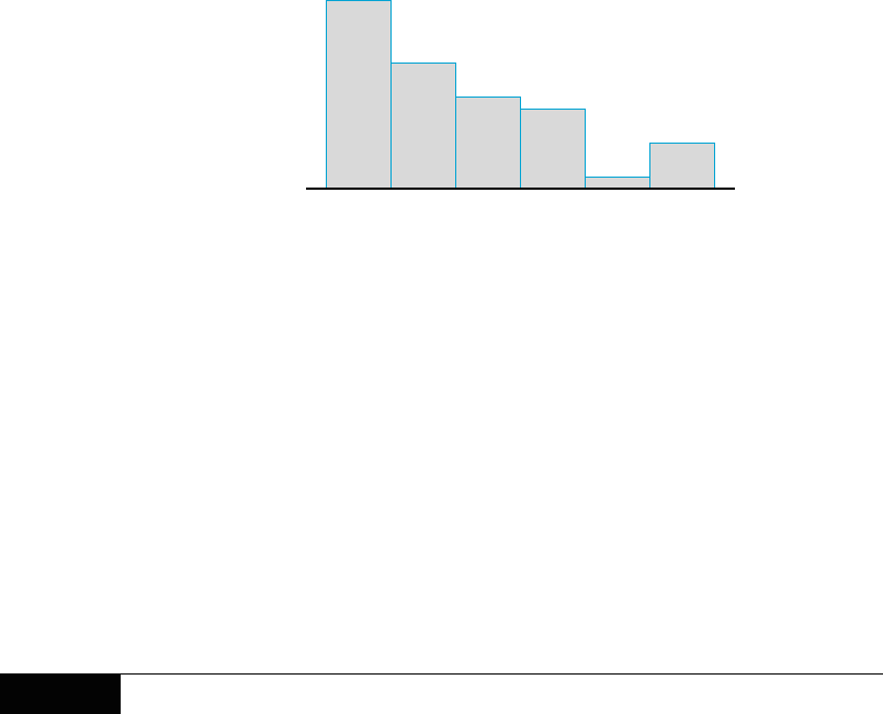
Example 1.10 Each member of a sample of 120 individuals owning motorcycles was asked for

the name of the manufacturer of his or her bike. The frequency distribution for the

resulting data is given in Table 1.2 and the histogram is shown in Figure 1.11.

abc d

Figure 1.10 Smoothed histograms: (a) symmetric unimodal; (b) bimodal; (c) positively skewed; and

(d) negatively skewed

Table 1.2 Frequency distribution for motorcycle data

Manufacturer Frequency Relative frequency

1. Honda 41 .34

2. Yamaha 27 .23

3. Kawasaki 20 .17

4. Harley-Davidson 18 .15

5. BMW 3 .03

6. Other 11 .09

120 1.01

1.2 Pictorial and Tabular Methods in Descriptive Statistics 19

Multivariate Data

The techniques presented so far have been exclusively for situations in which each

observation in a data set is either a single number or a sing le category. Often,

however, the data is multivariate in nature. That is, if we obtain a sample of

individuals or objects and on each one we make two or more measurements, then

each “observation” would consist of several measurements on one individual or

object. The sample is bivariate if each observation consists of two measurements

or responses, so that the data set can be represented as (x

, y

), ... ,(x

, y

). For

example, x might refer to engine size and y to horsepower, or x might refer to brand

of calculator owned and y to acade mic major. We briefly consider the analysis of

multivariate data in several later chapters.

Exercises Section 1.2 (10–29)

10. Consider the IQ data given in Example 1.2.

a. Construct a stem-and-leaf display of the data.

What appears to be a representative IQ value?

Do the observations appear to be highly con-

centrated about the representative value or

rather spread out?

b. Does the display appear to be reasonably sym-

metric about a representative value, or would

you describe its shape in some other way?

c. Do there appear to be any outlying IQ values?

d. What proportion of IQ values in this sample

exceed 100?

11. Every score in the following batch of exam

scores is in the 60’s, 70’s, 80’s, or 90’s.

A stem-and-leaf display with only the four

stems 6, 7, 8, and 9 would not give a very

detailed description of the distribution of scores.

In such situations, it is desirable to use repeated

stems. Here we could repeat the stem 6 twice,

using 6L for scores in the low 60’s (leaves 0, 1, 2,

3, and 4) and 6H for scores in the high 60’s

(leaves 5, 6, 7, 8, and 9). Similarly, the other

stems can be repeated twice to obtain a display

consisting of eight rows. Construct such a display

for the given scores. What feature of the data is

highlighted by this display?

74 89 80 93 64 67 72 70 66 85 89 81 81

71 74 82 85 63 72 81 81 95 84 81 80 70

69 66 60 83 85 98 84 68 90 82 69 72 87

12. The accompanying specific gravity values for

various wood types used in construction

appeared in the article “Bolted Connection

Design Values Based on European Yield

Model” (J. Struct. Engrg., 1993: 2169–2186):

.31 .35 .36 .36 .37 .38 .40 .40 .40

.41 .41 .42 .42 .42 .42 .42 .43 .44

.45 .46 .46 .47 .48 .48 .48 .51 .54

.54 .55 .58 .62 .66 .66 .67 .68 .75

.34

.23

.17

.15

.03

.09

(1) (2) (3) (4) (5) (6)

Figure 1.11 Histogram for motorcycle data ■

20 CHAPTER 1 Overview and Descriptive Statistics

Construct a stem-and-leaf display using repeated

stems (see the previous exercise), and comment

on any interesting features of the display.

13. The accompanying data set consists of observa-

tions on shower-flow rate (L/min) for a sample of

n ¼ 129 houses in Perth, Australia (“An Appli-

cation of Bayes Methodology to the Analysis of

Diary Records in a Water Use Study,” J. Amer.

Statist. Assoc., 1987: 705–711):

4.6 12.3 7.1 7.0 4.0 9.2 6.7 6.9 11.5 5.1

11.2 10.5 14.3 8.0 8.8 6.4 5.1 5.6 9.6 7.5

7.5 6.2 5.8 2.3 3.4 10.4 9.8 6.6 3.7 6.4

8.3 6.5 7.6 9.3 9.2 7.3 5.0 6.3 13.8 6.2

5.4 4.8 7.5 6.0 6.9 10.8 7.5 6.6 5.0 3.3

7.6 3.9 11.9 2.2 15.0 7.2 6.1 15.3 18.9 7.2

5.4 5.5 4.3 9.0 12.7 11.3 7.4 5.0 3.5 8.2

8.4 7.3 10.3 11.9 6.0 5.6 9.5 9.3 10.4 9.7

5.1 6.7 10.2 6.2 8.4 7.0 4.8 5.6 10.5 14.6

10.8 15.5 7.5 6.4 3.4 5.5 6.6 5.9 15.0 9.6

7.8 7.0 6.9 4.1 3.6 11.9 3.7 5.7 6.8 11.3

9.3 9.6 10.4 9.3 6.9 9.8 9.1 10.6 4.5 6.2

8.3 3.2 4.9 5.0 6.0 8.2 6.3 3.8 6.0

a. Construct a stem-and-leaf display of the data.

b. What is a typical, or representative, flow rate?

c. Does the display appear to be highly concen-

trated or spread out?

d. Does the distribution of values appear to be

reasonably symmetric? If not, how would you

describe the departure from symmetry?

e. Would you describe any observation as being

far from the rest of the data (an outlier)?

14. Do running times of American movies differ

somehow from times of French movies? The

authors investigated this question by randomly

selecting 25 recent movies of each type, resulting

in the following running times:

Am: 94 90 95 93 128 95 125

91 104 116 162 102 90 110

92 113 116 90 97 103 95

120 109 91 138

Fr: 123 116 90 158 122 119 125

90 96 94 137 102 105 106

95 125 122 103 96 111 81

113 128 93 92

Construct a comparative stem-and-leaf display

by listing stems in the middle of your paper and

then placing the Am leaves out to the left and the

Fr leaves out to the right. Then comment on

interesting features of the display.

15. Temperature transducers of a certain type are

shipped in batches of 50. A sample of 60 batches

was selected, and the number of transducers

in each batch not conforming to design specifi-

cations was determined, resulting in the follo-

wing data:

212401 32053313247023

042131 13412322845131

502321 06421603336123

a. Determine frequencies and relative frequen-

cies for the observed values of x ¼ number of

nonconforming transducers in a batch.

b. What proportion of batches in the sample have

at most five nonconforming transducers? What

proportion have fewer than five? What propor-

tion have at least five nonconforming units?

c. Draw a histogram of the data using relative

frequency on the vertical scale, and comment

on its features.

16. In a study of author productivity (“Lotka’s Test,”

Collection Manage., 1982: 111–118), a large

number of authors were classified according to

the number of articles they had published during

a certain period. The results were presented in

the accompanying frequency distribution:

Number of

papers 1 2 345678

Frequency 784 204 127 50 33 28 19 19

Number of

papers 9 10 11121314151617

Frequency 6 7 6744533

a. Construct a histogram corresponding to this

frequency distribution. What is the most inter-

esting feature of the shape of the distribution?

b. What proportion of these authors published at

least five papers? At least ten papers? More

than ten papers?

c. Suppose the five 15’s, three 16’s, and three

17’s had been lumped into a single category

displayed as “15.” Would you be able to

draw a histogram? Explain.

d. Suppose that instead of the values 15, 16, and

17 being listed separately, they had been com-

bined into a 15–17 category with frequency

11. Would you be able to draw a histogram?

Explain.

17. The article “Ecological Determinants of Herd

Size in the Thorncraft’s Giraffe of Zambia”

(Afric. J. Ecol., 2010: 962–971) gave the follow-

ing data (read from a graph) on herd size for a

sample of 1570 herds over a 34-year period.

Herd size 12345678

Frequency 589 190 176 157 115 89 57 55

Herd size 910111213141517

Frequency 33 31 22 10 4 10 11 5

Herd size 18 19 20 22 23 24 26 32

Frequency 24222211

1.2 Pictorial and Tabular Methods in Descriptive Statistics

a. What proportion of the sampled herds had just

one giraffe?

b. What proportion of the sampled herds had six

or more giraffes (characterized in the article

as “large herds”)?

c. What proportion of the sampled herds had

between five and ten giraffes, inclusive?

d. Draw a histogram using relative frequency on

the vertical axis. How would you describe the

shape of this histogram?

18. The article “Determination of Most Representa-

tive Subdivision” (J. Energy Engrg., 1993:

43–55) gave data on various characteristics of

subdivisions that could be used in deciding

whether to provide electrical power using over-

head lines or underground lines. Here are the

values of the variable x ¼ total length of streets

within a subdivision:

1280 5320 4390 2100 1240 3060 4770

1050 360 3330 3380 340 1000 960

1320 530 3350 540 3870 1250 2400

960 1120 2120 450 2250 2320 2400

3150 5700 5220 500 1850 2460 5850

2700 2730 1670 100 5770 3150 1890

510 240 396 1419 2109

a. Construct a stem-and-leaf display using the

thousands digit as the stem and the hundreds

digit as the leaf, and comment on the various

features of the display.

b. Construct a histogram using class boundaries

0, 1000, 2000, 3000, 4000, 5000, and 6000.

What proportion of subdivisions have total

length less than 2000? Between 2000 and

4000? How would you describe the shape of

the histogram?

19. The article cited in Exercise 18 also gave the

following values of the variables y ¼ number of

culs-de-sac and z ¼ number of intersections:

y 1010020111210011011

z 1861153004400121404

y 1100011201221102110

z 0301101324660118335

y 150301100

z 052310003

a. Construct a histogram for the y data. What

proportion of these subdivisions had no culs-

de-sac? At least one cul-de-sac?

b. Construct a histogram for the z data. What pro-

portion of these subdivisions had at most five

intersections? Fewer than five intersections?

20. How does the speed of a runner vary over the course

of a marathon (a distance of 42.195 km)? Consider

determining both the time to run the first 5 km and

the time to run between the 35-km and 40-km points,

and then subtracting the former time from the latter

time. A positive value of this difference corresponds

to a runner slowing down toward the end of the race.

The accompanying histogram is based on times of

runners who participated in several different Japa-

nese marathons (“Factors Affecting Runners’ Mar-

athon Performance,” Chance, Fall 1993: 24–30).

What are some interesting features of this

histogram? What is a typical difference value?

Roughly what proportion of the runners ran the

late distance more quickly than the early distance?

Histogram for Exercise 20

100

150

200

−100 100 200

Time

difference

300 400 500 600 700 800

Frequency

22 CHAPTER 1 Overview and Descriptive Statistics

21. In a study of warp breakage during the weaving of

fabric (Technometrics, 1982: 63), 100 specimens

of yarn were tested. The number of cycles of strain

to breakage was determined for each yarn speci-

men, resulting in the following data:

86 146 251 653 98 249 400 292 131 169

175 176 76 264 15 364 195 262 88 264

157 220 42 321 180 198 38 20 61 121

282 224 149 180 325 250 196 90 229 166

38 337 65 151 341 40 40 135 597 246

211 180 93 315 353 571 124 279 81 186

497 182 423 185 229 400 338 290 398 71

246 185 188 568 55 55 61 244 20 284

393 396 203 829 239 236 286 194 277 143

198 264 105 203 124 137 135 350 193 188

a. Construct a relative frequency histogram based

on the class intervals 0–100, 100–200, ..., and

comment on features of the distribution.

b. Construct a histogram based on the following

class intervals: 0–50, 50–100, 100–150,

150–200, 200–300, 300–400, 400–500,

500–600, 600–900.

c. If weaving specifications require a breaking

strength of at least 100 cycles, what proportion

of the yarn specimens in this sample would be

considered satisfactory?

22. The accompanying data set consists of observa-

tions on shear strength (lb) of ultrasonic spot

welds made on a type of alclad sheet. Construct

a relative frequency histogram based on ten equal-

width classes with boundaries 4000, 4200, ... .

[The histogram will agree with the one in “Com-

parison of Properties of Joints Prepared by Ultra-

sonic Welding and Other Means” (J. Aircraft,

1983: 552–556).] Comment on its features.

5434 4948 4521 4570 4990 5702 5241

5112 5015 4659 4806 4637 5670 4381

4820 5043 4886 4599 5288 5299 4848

5378 5260 5055 5828 5218 4859 4780

5027 5008 4609 4772 5133 5095 4618

4848 5089 5518 5333 5164 5342 5069

4755 4925 5001 4803 4951 5679 5256

5207 5621 4918 5138 4786 4500 5461

5049 4974 4592 4173 5296 4965 5170

4740 5173 4568 5653 5078 4900 4968

5248 5245 4723 5275 5419 5205 4452

5227 5555 5388 5498 4681 5076 4774

4931 4493 5309 5582 4308 4823 4417

5364 5640 5069 5188 5764 5273 5042

5189 4986

23. A transformation of data values by means of some

mathematical function, such as

ﬃﬃﬃ

or 1/x, can often

yield a set of numbers that has “nicer” statistical

properties than the original data. In particular, it

may be possible to find a function for which the

histogram of transformed values is more symmetric

(or, even better, more like a bell-shaped curve) than

the original data. As an example, the article “Time

Lapse Cinematographic Analysis of Beryllium–

Lung Fibroblast Interactions” (Environ. Res.,

1983: 34–43) reported the results of experiments

designed to study the behavior of certain individual

cells that had been exposed to beryllium. An impor-

tant characteristic of such an individual cell is its

interdivision time (IDT). IDTs were determined for

a large number of cells both in exposed (treatment)

and unexposed (control) conditions. The authors of

the article used a logarithmic transformation, that is,

transformed value ¼ log

(original value). Con-

sider the following representative IDT data:

28.1 31.2 13.7 46.0 25.8 16.8 34.8

62.3 28.0 17.9 19.5 21.1 31.9 28.9

60.1 23.7 18.6 21.4 26.6 26.2 32.0

43.5 17.4 38.8 30.6 55.6 25.5 52.1

21.0 22.3 15.5 36.3 19.1 38.4 72.8

48.9 21.4 20.7 57.3 40.9

Use class intervals 10–20, 20–30, ... to construct a

histogram of the original data. Use intervals 1.1–1.2,

1.2–1.3, ...to do the same for the transformed data.

What is the effect of the transformation?

24. Unlike most packaged food products, alcohol bev-

erage container labels are not required to show

calorie or nutrient content. The article “What Am

I Drinking? The Effects of Serving Facts Informa-

tion on Alcohol Beverage Containers” (J. of

Consumer Affairs, 2008: 81–99) reported on a

pilot study in which each individual in a sample

was asked to estimate the calorie content of a 12 oz

can of light beer known to contain 103 cal. The

following information appeared in the article:

Class Percentage

0–<50 7

50 – < 75 9

75 – < 100 23

100 – < 125 31

125 – < 150 12

150 – < 200 3

200 – < 300 12

300 – < 500 3

a. Construct a histogram of the data and comment

on any interesting features.

b. What proportion of the estimates were at least

100? Less than 200?

1.2 Pictorial and Tabular Methods in Descriptive Statistics 23

25. The article “Study on the Life Distribution of

Microdrills” (J. Engrg. Manuf., 2002: 301–305)

reported the following observations, listed in

increasing order, on drill lifetime (number of

holes that a drill machines before it breaks) when

holes were drilled in a certain brass alloy.

11 14 20 23 31 36 39 44 47 50

59 61 65 67 68 71 74 76 78 79

81 84 85 89 91 93 96 99 101 104

105 105 112 118 123 136 139 141 148 158

161 168 184 206 248 263 289 322 388 513

a. Construct a frequency distribution and histo-

gram of the data using class boundaries 0, 50,

100, ... , and then comment on interesting

characteristics.

b. Construct a frequency distribution and histo-

gram of the natural logarithms of the lifetime

observations, and comment on interesting

characteristics.

c. What proportion of the lifetime observa-

tions in this sample are less than 100?

What proportion of the observations are at

least 200?

26. Consider the following data on type of health com-

plaint (J ¼ joint swelling, F ¼ fatigue, B ¼ back

pain, M ¼ muscle weakness, C ¼ coughing, N ¼

nose running/irritation, O ¼ other) made by tree

planters. Obtain frequencies and relative frequen-

cies for the various categories, and draw a histo-

gram. (The data is consistent with percentages

given in the article “Physiological Effects of

Work Stress and Pesticide Exposure in Tree Plant-

ing by British Columbia Silviculture Workers,”

Ergonomics, 1993: 951–961.)

OONJ CFBBF OJ O OM

OF F OONONJ F J B OC

JOJJFNOBMOJMOB

OF J OOBNCO OOMBF

JOFN

27. A Pareto diagram is a variation of a histogram for

categorical data resulting from a quality control

study. Each category represents a different type of

product nonconformity or production problem. The

categories are ordered so that the one with the

largest frequency appears on the far left, then the

category with the second largest frequency, and so

on. Suppose the following information on noncon-

formities in circuit packs is obtained: failed com-

ponent, 126; incorrect component, 210; insufficient

solder, 67; excess solder, 54; missing component,

131. Construct a Pareto diagram.

28. The cumulative frequency and cumulative rela-

tive frequency for a particular class interval are

the sum of frequencies and relative frequencies,

respectively, for that interval and all intervals

lying below it. If, for example, there are four

intervals with frequencies 9, 16, 13, and 12, then

the cumulative frequencies are 9, 25, 38, and

50, and the cumulative relative frequencies are

.18, .50, .76, and 1.00. Compute the cumulative

frequencies and cumulative relative frequencies

for the data of Exercise 22.

29. Fire load (MJ/m

) is the heat energy that could be

released per square meter of floor area by com-

bustion of contents and the structure itself. The

article “Fire Loads in Office Buildings” (J. Struct.

Engrg., 1997: 365–368) gave the following cumu-

lative percentages (read from a graph) for fire

loads in a sample of 388 rooms:

Value 0 150 300 450 600

Cumulative % 0 19.3 37.6 62.7 77.5

Value 750 900 1050 1200 1350

Cumulative % 87.2 93.8 95.7 98.6 99.1

Value 1500 1650 1800 1950

Cumulative % 99.5 99.6 99.8 100.0

a. Construct a relative frequency histogram and

comment on interesting features.

b. What proportion of fire loads are less than 600?

At least 1200?

c. What proportion of the loads are between 600

and 1200?

1.3

Measures of Location

Visual summaries of data are excellent tools for obtaining preliminary impressions

and insights. More formal data anal ysis often requires the calculation and interpre-

tation of numerical summary measures. That is, from the data we try to extract

several summarizing numbers —numbers that might serve to characterize the data

set and convey some of its mos t important features. Our primary concern will be

with numerical data; some comments regarding cat egorical data appear at the end

of the section.

24 CHAPTER 1 Overview and Descriptive Statistics

Suppose, then, that our data set is of the form x

, x

, ..., x

, where each x

is a

number. What features of such a set of numbers are of most interest and deserve

emphasis? One important characteristic of a set of numbers is its location, and in

particular its center. This section presents methods for descr ibing the location of a

data set; in Section 1.4 we will turn to methods for measuring variability in a set of

numbers.

The Mean

For a given set of numbers x

, x

, ..., x

, the most familiar and useful measure of

the center is the mean, or arithmeti c average of the set. Because we will almost

always think of the x

’s as constituting a sample, we will often refer to the

arithmetic average as the sample mean and denote it by



DEFINITION

The sample mean



x of observations x

, x

, ... , x

is given by



x ¼

þ x

þþx

i¼1

The numerator of



x can be written more informally as

where the

summation is over all sample observations.

For reporting



x, we recommend using decimal accuracy of one digit more than the

accuracy of the x

’s. Thus if observations are stopping distances with x

¼ 125,

¼ 131, and so on, we might have



x ¼ 127:3 ft.

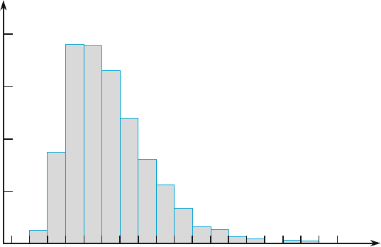
Example 1.11 A class was assigned to make wingspan measurements at home. The wingspan is

the horizontal measurement from fingertip to fingertip with outstretched arms. Here

are the measurements given by 21 of the students.

¼ 60 x

¼ 64 x

¼ 72 x

¼ 63 x

¼ 66 x

¼ 62 x

¼ 75

¼ 66 x

¼ 59 x

¼ 75 x

¼ 69 x

¼ 62 x

¼ 63 x

¼ 61

¼ 65 x

¼ 67 x

¼ 65 x

¼ 69 x

¼ 95 x

¼ 60 x

¼ 70

Figure 1.12 shows a stem-and-leaf display of the data; a wingspan in the 60’s

appears to be “typical.”

5H|9

6L|00122334

6H|5566799

7L|02

7H|55

8L|

8H|

9L|

9H|5

Figure 1.12 A stem-and-leaf display of the wingspan data

1.3 Measures of Location 25

With

¼ 1408, the sample mean is



x ¼

1408

¼ 67:0

a value consistent with information conveyed by the stem-and-leaf display.

■

A physical interpretation o f



x dem onstrates how it measures the location

(center) of a sample. Think of drawing and scaling a horizontal measurement axis,

and then representing each sample observation by a 1-lb weight placed at the

corresponding point on the axis. The only point at which a fulcrum can be placed

to balance the system of weights is the point corresponding to the value of



x (see

Figure 1.13). The system balances because, as shown in the next section,

ðx





xÞ¼0 so the net total tendency to turn about



x is 0.

Just as



x repr esents the average value of the observations in a sample, the

average of all values in the population can in principle be calculated. This average

is called the population mean and is denoted by the Greek letter m. When there are

N valu es in the population (a finite population), then m ¼ (sum of the N population

values)/N. In Chapters 3 and 4, we will give a more general definition for m that

applies to both finite and (conceptually) infinite populations. Just as



x is an

interesting and important measure of sample location, m is an interesting and

important (often the most important) characteristic of a population. In the chapters

on statistical inference, we will present methods based on the sample mean for

drawing conclusions about a population mean. For example, we might use the

sample mean



x ¼ 67:0 computed in Example 1.11 as a point estimate (a single

number that is our “best” guess) of m ¼ the true average wingspan for all students

in introductory statistics classes.

The mean suffers from one deficiency that makes it an inappropriate measure

of center under some circumstances: its value can be greatly affected by the

presence of even a single outlier (unusually large or small observation). In Example

1.11, the value x

¼ 95 is obvio usly an outlier. Without this observation,



x ¼ 1313=20 ¼ 65:7; the o utlier increases the mean by 1.3 in. The value 95 is

clearly an error—this student is only 70 in. tall, and there is no way such a student

could have a wingspan of almost 8 ft. As Leonardo da Vinci noticed, wingspan is

usually quite close to height.

Data on housing prices in various metropolitan areas often contains outliers

(those lucky enough to live in palatial accommodations), in whi ch case the use of

average price as a measure of center will typically be misleading. We will momen-

tarily propose an alternative to the mean, namely the median, that is insensitive to

outliers (recent New York City data gave a median price of less than $700,000 and

a mean price exceeding $1,000,000). Howeve r, the mean is still by far the most

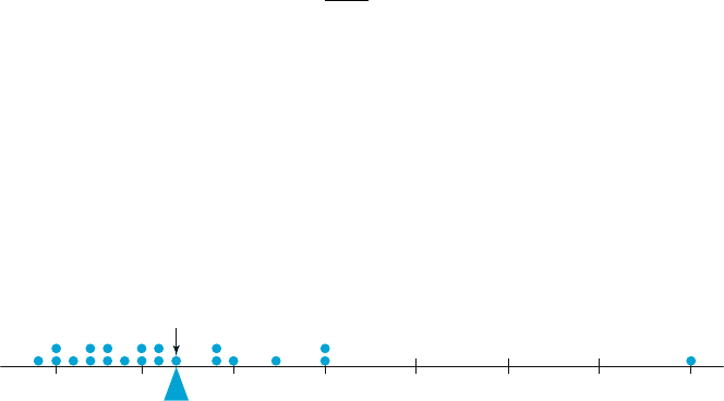
60 65 70 75 80 85 90 95

Mean = 67.0

Figure 1.13 The mean as the balance point for a system of weights

CHAPTER 1 Overview and Descriptive Statistics

widely used measure of center, largely because there are many populations for

which outliers are very scarce. When sampling from such a population (a normal or

bell-shaped distribution being the most important example), outliers are highly

unlikely to enter the sample. The sample mean will then tend to be stable and quite

representative of the sample.

The Median

The word median is synonymous with “middle,” and the sample median is indeed

the middle value when the observations are ordered from smallest to largest. When

the observations are denoted by x

, ..., x

, we will use the symbol

x to represent the

sample median.

DEFINITION

The sample median is obtained by first ordering the n observations from

smallest to largest (with any repeated values included so that every sample

observation appears in the ordered list). Then,

x ¼

The single

middle

value if n

is odd

n þ1



ordered value

The average

of the two

middle

values if n

is even

¼average of



and

þ1



ordered values

Example 1.12 People not familiar with classical music might tend to believe that a composer’s

instructions for playing a particular piece are so specific that the duration would not

depend at all on the performer(s). However, there is typicall y plenty of room for

interpretation, and orchestral conductors and musicians take full advantage of this.

We went to the website ArkivMusic.com and selected a sample of 12 recordings of

Beethoven’s Symphony #9 (the “Choral”, a stunningly beautiful work), yielding

the following durations (min) listed in increasing order:

62.3 62.8 63.6 65.2 65.7 66.4 67.4 68.4 68.8 70.8 75.7 79.0

Since n ¼ 12 is even, the sample median is the average of the n/2 ¼ 6th and

(n/2 + 1) ¼ 7th values from the ordered list:

x ¼

66:4 þ 67:4

¼ 66:90

1.3 Measures of Location 27