Devore J.L., Berk K.N. Modern Mathematical Statistics with Applications

Подождите немного. Документ загружается.

37. The n ¼ 26 observations on escape time given in

Exercise 33 of Chapter 1 give a sample mean and

sample standard deviation of 370.69 and 24.36,

respectively.

a. Calculate an upper confidence bound for pop-

ulation mean escape time using a confidence

level of 95%.

b. Calculate an upper prediction bound for the

escape time of a single additional worker

using a prediction level of 95%. How does

this bound compare with the confidence

bound of part (a)?

c. Suppose that two additional workers will be

chosen to participate in the simulated escape

exercise. Denote their escape times by X

and

, and let X

new

denote the average of these

two values. Modify the formula for a PI for a

single x value to obtain a PI for

new

, and

calculate a 95% two-sided interval based on

the given escape data.

38. A study of the ability of individuals to walk in a

straight line (“Can We Really Walk Straight?”

Amer. J. Phys. Anthropol., 1992: 19–27) reported

the accompanying data on cadence (strides per

second) for a sample of n ¼ 20 randomly selected

healthy men.

.95 .85 .92 .95 .93 .86 1.00 .92 .85 .81

.78 .93 .93 1.05 .93 1.06 1.06 .96 .81 .96

A normal probability plot gives substantial sup-

port to the assumption that the population distri-

bution of cadence is approximately normal. A

descriptive summary of the data from MINITAB

follows:

Variable N Mean Median TrMean StDev SEMean

Cadence 20 0.9255 0.9300 0.9261 0.0809 0.0181

Variable Min Max Q1 Q3

Cadence 0.7800 1.0600 0.8525 0.9600

a. Calculate and interpret a 95% confidence inter-

val for population mean cadence.

b. Calculate and interpret a 95% prediction inter-

val for the cadence of a single individual ran-

domly selected from this population.

39. A sample of 25 pieces of laminate used in the

manufacture of circuit boards was selected and

the amount of warpage (in.) under particular con-

ditions was determined for each piece, resulting in

a sample mean warpage of .0635 and a sample

standard deviation of .0065. Calculate a prediction

for the amount of warpage of a single piece of

laminate in a way that provides information about

precision and reliability.

40. Exercise 69 of Chapter 1 gave the following

observations on a receptor binding measure

(adjusted distribution volume) for a sample of 13

healthy individuals: 23, 39, 40, 41, 43, 47, 51, 58,

63, 66, 67, 69, 72.

a. Is it plausible that the population distribution

from which this sample was selected is nor-

mal?

b. Predict the adjusted distribution volume of a

single healthy individual by calculating a 95%

prediction interval.

41. Here are the lengths (in minutes) of the 63 nine-

inning games from the first week of the 2001

major league baseball season:

194 160 176 203 187 163 162 183 152 177

177 151 173 188 179 194 149 165 186 187

187 177 187 186 187 173 136 150 173 173

136 153 152 149 152 180 186 166 174 176

198 193 218 173 144 148 174 163 184 155

151 172 216 149 207 212 216 166 190 165

176 158 198

Assume that this is a random sample of nine-

inning games (the mean differs by 12 s from the

mean for the whole season).

a. Give a 95% confidence interval for the popula-

tion mean.

b. Give a 95% prediction interval for the length of

the next nine-inning game. On the first day of

the next week, Boston beat Tampa Bay 3–0 in

a nine-inning game of 152 min. Is this within

the prediction interval?

c. Compare the two intervals and explain why one

is much wider than the other.

d. Explore the issue of normality for the data and

explain how this is relevant to parts (a) and (b).

42. A more extensive tabulation of t critical values

than what appears in this book shows that for the

t distribution with 20 df, the areas to the right of

the values .687, .860, and 1.064 are .25, .20, and

.15, respectively. What is the confidence level for

each of the following three confidence intervals

for the mean m of a normal population distribu-

tion? Which of the three intervals would you rec-

ommend be used, and why?

a. ð

x  :687s=

ﬃﬃﬃﬃﬃ

; x þ 1:725s=

ﬃﬃﬃﬃﬃ

b. ð

x  :860s=

ﬃﬃﬃﬃﬃ

; x þ 1:325s=

ﬃﬃﬃﬃﬃ

c. ð

x  1:064s=

ﬃﬃﬃﬃﬃ

; x þ 1:064s=

ﬃﬃﬃﬃﬃ

43. Use the results of Section 6.4 to show that the

variable T on which the PI is based does in fact

have a t distribution with n  1 df.

408

CHAPTER 8 Statistical Intervals Based on a Single Sample

8.4

Confidence Intervals for the Variance

and Standard Deviation of a Normal

Population

Although inferences concerning a population varianc e s

or standard deviation

s are usually of less interest than those about a mean or proportion, there are

occasions when such procedures are needed. In the case of a normal population

distribution, inferences are based on the following result from Section 6.4

concerning the sample variance S

THEOREM

Let X

, X

, ... , X

be a random sample from a normal distribution with

parameters m and s

. Then the rv

ðn  1ÞS

ðX

 XÞ

has a chi-squared (w

) probability distribution with n  1 df.

As disc ussed in Sections 4.4 and 6.4, the chi-squared distribution is a continu-

ous probability distribution with a single parameter n, the number of degrees of

freedom, with possible values 1, 2, 3, .... To specify inferential procedures that use

the chi-squared distribution, recall the notation for critical values from Section 6.4.

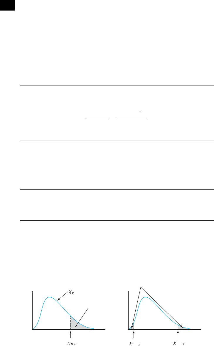
NOTATION

Let w

a;n

, called a chi-squared critical value, denote the number on the

measurement axis such that a of the area under the chi-squared curve with

n df lies to the right of w

a;n

Because the t distribution is symmetric, it was necessary to tabulate only

upper-tail critica l values (t

a,n

for small values of a). The chi-squared distribution is

not symmetric, so Appendix Table A.6 contains values of w

a;n

for a both near 0 and

near 1, as illustrated in Figure 8.9(b). For example, w

:025;14

¼ 26:119 and w

:95;20

(the

5th percentile) ¼ 10.851.

pdf

Shaded area = a

.99,

.01,

Each shaded

area = .01

Figure 8.9 w

a;u

notation illustrated

8.4 Conﬁdence Intervals for the Variance and Standard Deviation of a Normal Population 409

The rv (n  1)S

satisfies the two properties on which the general method

for obtaining a CI is based: It is a function of the parameter of interest s

, yet its

probability distribution (chi-squared) does not depend on this parameter. The area

under a chi- squared curve with n df to the rig ht of w

a=2;n

is a/2, as is the area to the

left of w

1a=2;n

. Thus the area captured between these two critical values is 1  a.

As a consequence of this and the theorem just stated,

P w

1a=2;n1

ðn  1ÞS

< w

a=2;n1



¼ 1  a ð8:17Þ

The inequalities in (8.17) are equivalent to

ðn  1ÞS

a=2;n1

< s

ðn  1ÞS

1a=2;n1

Substituting the computed value s

into the limits gives a CI for s

, and taking

square roots gives an interval for s.

A 100(1  a)% confidence interval for the variance s

of a normal

population has lower limit

ðn  1Þs

a=2;n1

and upper limit

ðn  1Þs

1a=2;n1

A confidence interval for s has lower and upper limits that are the square

roots of the corresponding limits in the interval for s

Example 8.14 Recall the beer alcohol percentage data from Example 8.11, where the normal plot

was acceptably straight and the standard deviation was found to be s ¼ .8483.

Then the sample variance is s

¼ .8483

¼ .7196, and we wish to estimate the

population variance s

. With df ¼ n  1 ¼ 15, a 95% confidence interval requires

:975;15

¼ 6:262 and w

:025;15

¼ 27:488. The interval for s

15ð:7196Þ

27:488

;

15ð:7196Þ

6:262



¼ð:393; 1:724Þ

Taking the square root of each endpoint yields (.627, 1.313) as the 95% confidence

interval for s. With lower and upper limits differing by more than a factor of two,

this interval is quite wide. Precise estimat es of variability require large samples.

■

Unfortunately, our confidence interval requires that the data be normal or nearly

normal. In the case of nonnormal data the interval could be very far from valid; for

example, the true confidence level could be 70% where 95% is intended. See Exercise

57 in the next section for a method that does not require the normal distribution.

410 CHAPTER 8 Statistical Intervals Based on a Single Sample

Exercises Section 8.4 (44–48)

44. Determine the values of the following quantities:

a. w

:1;15

b. w

:1;25

c. w

:01;25

d. w

:005;25

e. w

:99;25

f. w

:995;25

45. Determine the following:

a. The 95th percentile of the chi-squared distribu-

tion with n ¼ 10

b. The 5th percentile of the chi-squared distribu-

tion with n ¼ 10

c. P(10.98  w

 36.78), where w

is a chi-

squared rv with n ¼ 22

d. P(w

< 14.611 or w

> 37.652), where w

is a

chi-squared rv with n ¼ 25

46. Exercise 34 gave a random sample of 20 ACT

scores from students taking college freshman calcu-

lus. Calculate a 99% CI for the standard deviation of

the population distribution. Is this interval valid

whatever the nature of the distribution? Explain.

47. Here are the names of 12 orchestra conductors and

their performance times in minutes for Beetho-

ven’s Ninth Symphony:

Bernstein 71.03 Furtw

€

angler 74.38

Leinsdorf 65.78 Ormandy 64.72

Solti 74.70 Szell 66.22

Bohm 72.68 Karajan 66.90

Masur 69.45 Rattle 69.93

Steinberg 68.62 Tennstedt 68.40

a. Check to see that normality is a reasonable

assumption for the performance time distribu-

tion.

b. Compute a 95% CI for the population standard

deviation, and interpret the interval.

c. Supposedly, classical music is 100% deter-

mined by the composer’s notation, including

all timings. Based on your results, is this true

or false?

48. Refer to the baseball game times in Exercise 41.

Calculate an upper confidence bound with

confidence level 95% for the population

standard deviation of game time. Interpret your

interval. Explore the issue of normality for the

data and explain how this is relevant to your

interval.

8.5

Bootstrap Confidence Intervals

How can we find a confidence interval for the mean if the population distribution is

not normal and the sample size n is not large? Can we find confidence intervals for

other parameters such as the population median or the 90th percentile of the

population distribution? The bootstrap, developed by Bradley Efron in the late

1970s, allows us to calculate estimates in situations where statistical theory does

not produce a formula for a confidence interval. The method substitutes heavy

computation for theory, and it has been feasible only fairly recently with the

availability of fast computers. The bootstrap was introduced in Section 7.1 for

applications with known distribution (the parametri c bootstrap), but here we are

concerned with the case of unknown distribution (the nonparametric bootstrap).

Example 8.15 In a student project, Erich Brandt studied tips at a restaurant. Here is a random

sample of 30 observed tip percentages:

22.7, 16.3, 13.6, 16.8, 29.9, 15.9, 14.0, 15.0, 14.1, 18.1, 22.8, 27.6, 16.4, 16.1, 19.0,

13.5, 18.9, 20.2, 19.7, 18.2, 15.4, 15.7, 19.0, 11.5, 18.4, 16.0, 16.9, 12.0, 40.1, 19.2

We would like to get a confidence interval for the population mean tip percentage at

this restaurant. However, this is not a large sample and there is a problem with

positive skewness, as shown in the normal probability plot of Figure 8.10.

8.5 Bootstrap Conﬁdence Intervals 411

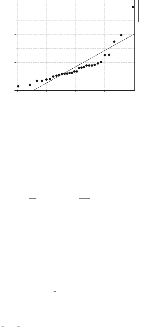
Most of the tips are between 10% and 20%, but a few big tips cause enough

skewness to invalidate the normality assumption. The sample mean is 18.43% and

the sample standard deviation is 5.76%.

If population normality were plausible, then we could form a confidence

interval using the mean and standard deviation calculated from the sample. From

Section 8.3, the resulting 95% confidence interval for the population mean would

x  t

:025;n1

ﬃﬃﬃ

¼ 18:43  2:045

5:76

ﬃﬃﬃﬃﬃ

¼ 18:43  2:15 ¼ð16 :3; 20:6Þ

How does the bootstrap approach differ from this? For the moment, we

regard the 30 obser vations as constituting a population, and take a large number

of random samples (999 is a common choice), each of size 30, from this population.

These are sample s with replacement, so repetitions are allowed. For each of these

samples we compute the mean (or the median or whatever statistic estimates the

population parameter). Then we use the distribution of these 999 means to get a

confidence interval for the population mean. To help get a feeling for how this

works, here is the first of the 999 samples:

22.8, 16.8, 16.0, 19.0, 19.2, 20.2, 13.6, 15.9, 22.8, 11.5, 15.9, 14.0, 29.9, 19.2, 16.0,

27.6, 14.1, 13.5, 16.8, 15.4, 20.2, 16.4, 20.2, 16.9, 16.8, 22.8, 19.7, 18.2, 22.7, 18.2

This sample has mean x



¼ 18:41, where the asterisk emphasizes that this is

the mean of a bootstrap sample.

Of course, when we take a random sample with replaceme nt, repetitions

usually occur as they do here, and this implies that not all of the 30 observations

will appear in each sample. After doing this 998 more times and computing the

means



; :::; x



999

for these 999 samples, we construct Figure 8.11, the histogram of

the 999



values.

−2 −1102

N30

Tip Percentage

z Score

Mean

StDev

P-Value

18.43

5.761

1.828

<0.005

Figure 8.10 Normal probability plot from MINITAB of the tip percentages

412

CHAPTER 8 Statistical Intervals Based on a Single Sample

This describ es approximately the sampling distribution of X for samples of 30

from the true tip population. That is, if we could draw the pdf for the true population

distribution of

x values, then it should look something like the histogram in

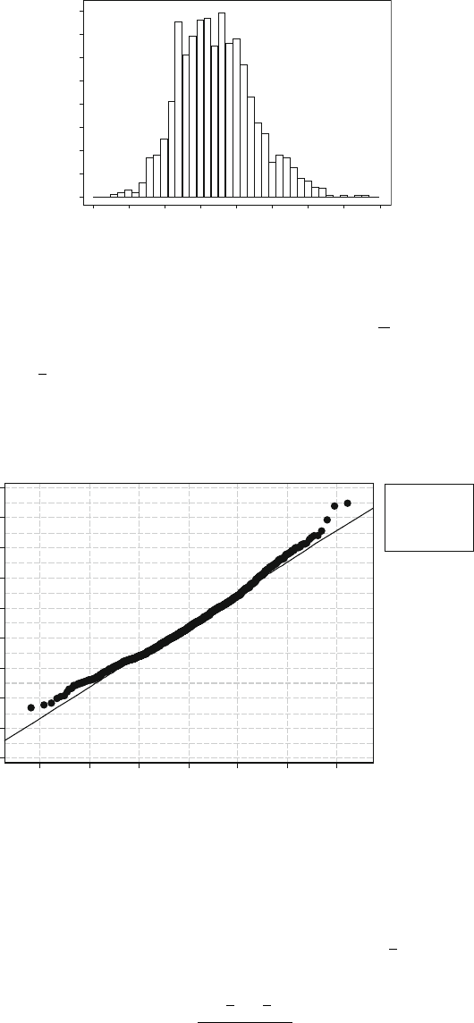
Figure 8.11. Does the distribution appear to be normal? The histogram is not

exactly symmetric, and the distribution looks skewed to the right. Figure 8.12 has

the normal probability plot from MINITAB:

The pattern in this plot gives evidence of slight positive skewnes s (see

Section 4.6). If this plot were straighter, then we could form a 9 5% confidence

interval for the population mean in the following way. Let s

boot

denote the sample

standard deviation of the 999 bootstrap means. That is, defining



to be the mean

of the 999 bootstrap means,

boot



 x



999  1

17 232016 2219

2118

Boot Tips

Frequency

Figure 8.11 Histogram of the tip bootstrap distribution, from MINITAB

−3 −2 −11230

N999

Mean

StDev

P-Value

18.46

1.043

3.101

<0.005

Boot Tips

z Score

Figure 8.12 Normal plot of the tip bootstrap distribution

8.5 Bootstrap Conﬁdence Intervals 413

The value of s

boot

turns out to be 1.043. The sample mean of the original 30 tip

percentages is

x ¼ 18:43, giving the 95% confidence interval

x  z

:025

boot

¼ 18:43  1:96ð 1 :043Þ¼18:43  2:04 ¼ð16:4; 20:5Þ

Notice that this is very similar to the previous interval based on the method of

Section 8.3. The difference is mainly due to using the z critical value instead of the

t critical value, because the bootstrap standard deviation s

boot

¼ 1.043 is close to

the estimated standard error s=

ﬃﬃﬃ

¼ 1:052. There should be good agreem ent if the

original data set looks normal. Even if the normality assumpt ion is not satisfied,

there should be good agreement if the sample size n is big enough.

■

The Percentile Interval

In the case that the bootstrap distribution (as represented here by the histogram of

Figure 8.11) is n ormal, the foregoing interval uses the middle 95% of the bootstrap

distribution. Because the 999 bootstrap means do not fit a normal curve, we need an

alternative approach to finding a confidence interval. To allow for a nonnormal

bootstrap distribution, we need to use something other than the standard deviation

and the t table to determine the confidence limits. The percentile interval uses the

2.5 percentile and the 97.5 percentile of the bootstrap distribution for confidence

limits of a 95% confidence interval. Computationally, one way to find the two

percentiles is to sort the 999 means and then use the 25th value from each end.

DEFINITION

The bootstrap percentile interval with a confidence level of 100(1  a)%

for a specified parameter is obtained by first generating B boots trap

samples, for each one calculating the value of some particular statistic that

estimates the para meter, and sorting these values from smallest to largest.

Then we compute k ¼ a(B + 1)/2 and choose the kth value from each end

of the sorted list. These two values form the confiden ce limits for the

confidence interval. If k is not an integer, then interpolation can be used,

but this is not crucial. As an example, if a ¼ .05 and B ¼ 999, then

k ¼ a(B + 1)/2 ¼ (.05)(999 + 1)/2 ¼ 25.

Example 8.16

(Example 8.15

continued)

For the tip data the 2.5 percentile is 16.7 and the 97.5 percentile is 20.8, so the 95%

bootstrap percentile interval (16.65, 20.80). Because the bootstrap distribution is

positively skewed, the percentile interval is shifted slightly to the right compared to

the interval based on a normal bootstrap distribution.

■

A Reﬁned Interval

When the percentile method is used to obtain a confidence interval, under some

circumstances the actual confidence level may differ substantially from the nomi-

nal level (the level you think you are getting); in our example, the nominal level

was 95%, and the actual level could be quite different from this. There are refined

bootstrap intervals that often yield an improvement in this respect. In particular,

414 CHAPTER 8 Statistical Intervals Based on a Single Sample

the BCa (bias corrected and accelerated) interval, implemented in the R, Stata, and

Systat software packa ges, is a method that corrects for bias . Here bias refers to the

difference between the mean of the bootstrap distribution compared to the value of

the estimate based on the original sample. For example, in estimating the mean for

the tip data, the mean of the 30 tips in the original sample is 18.43 but the mean of

the 999 bootstrap sample means is 18.46, so there is just a slight bias of

18.46  18.43 ¼ .03.

The acceleration aspect of the BCa interval is an adjustment for dependence

of the standard error of the estimator on the parameter that is being estimated. For

example, suppose we are trying to estimate the mean in the case of exponential

data. In this case the standard deviation is equal to the mean, and the standard error

X is s=

ﬃﬃﬃ

¼ m=

ﬃﬃﬃ

, so the standard error of the estimator X depends strongly on

the parameter m that is being estimated. If the histogram in Figure 8.11 resembled

the exponential pdf, we would expect the BCa method to make a substantial

correction to the percentile interval.

Example 8.17

(Example 8.16

continued)

Recall that the percentile interval for the mean of the tip data is (16.7, 20.8).

Compared to this, the BCa interval (16.9, 21.8) is shifted a little to the right.

■

Is the bootstrap guaranteed to work, or is it possible that the method can give

grossly incorrect estimates? The key here is how closely the original sample

represents the whole distribution of the random variable X. When the sample is

small, then there is a possibility that important features of the distribution are not

included in the data set. In terms of our 30 observations, the value 40.1% is highly

influential. If we drew another sample of 30 observations independent of this

sample, the luck of the draw might give no values above 25, and the sample

would yield very different conclusions. The bootstrap is a useful method for

making inferences from data, but it is dependent on a good sample. If this is all

the data that we can get, we will never know how well our sample represents the

distribution, and therefore how good our answer is. Of course, no statistical method

will give good answers if the sample is not representative of the population.

Bootstrapping the Median

We do have a statistic that is less sensitive to the influence of individual observa-

tions. For the 30 tip percent ages, the median is 16.85, substantially less than the

mean of 18.43. The mean is pulled upward by the few large values, but these

extremes have little effect on the median. In general, the median is less affected by

outliers than the mean. However, it is more difficult to get confidence intervals for

the median. There is a nice statistic to estimate the standard deviation of the mean

ðS=

ﬃﬃﬃ

Þ, but unfortunately there is nothing like this for the median.

Example 8.18

(Example 8.15

continued)

Let’s use the bootstrap method to get a confi dence interval for the median of the tip

data. We can use the same 999 samples of 30 as we did previously, but now we

instead look at the 999 medians. The first sample has mean



¼ 18:41, whereas its

median is



¼ 17:55. The histogram of this and the other 998 bootstrap medians



; ...;



999

is shown in Figure 8.13.

8.5 Bootstrap Conﬁdence Intervals 415

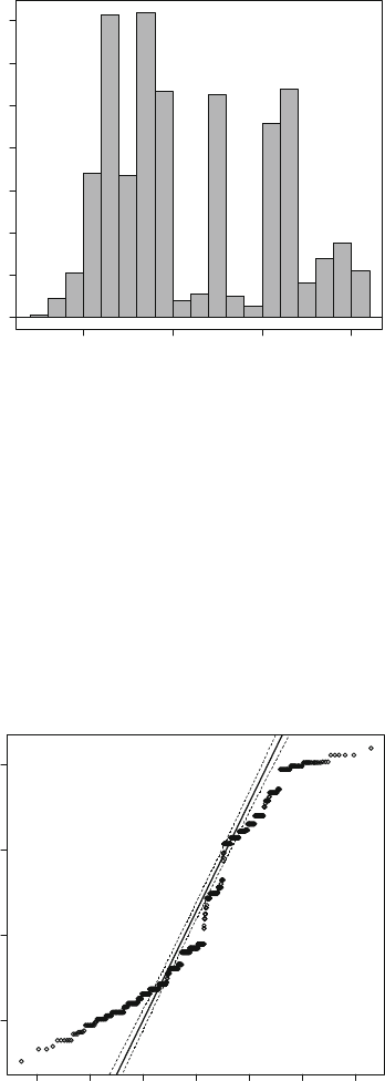
It should be apparent that the distribution of the 999 bootstrap medians is not

normal. As is often the case with the median, the boots trap distribution takes on just

a few values and there are many repeats. Instead of 999 different values, as would

be expected if we took 999 samples from a true continuous distribution, here there

are only 72 values, and some appear mor e than 50 times. These are apparent in the

normal probability plot, shown in Figure 8.14. In contrast to what MINITAB does,

the values here are plotted vertically, so the horizontal segments indicate repeats.

The mean of the 999 bootstrap medians is 17.20 with standard deviation .917.

Even though the procedure is inappropriate because of nonnormality, we can for

comparative purposes use the median

x ¼ 16:85 of the original 30 observations

Boot Median

frequency

16 17 18 19

140

120

100

Figure 8.13 Histogram of the bootstrap medians from R

−3 −2 −10

norm quantiles

Boot Median

Figure 8.14 Normal probability plot of the bootstrap medians from R

416

CHAPTER 8 Statistical Intervals Based on a Single Sample

together with the bootstrap standard deviation

boot

¼ :917 to get a confidence

interval based on the normal distribution:

x  z

:025

boot

¼ 16:85  1:96ð :917Þ¼16:85  1:80 ¼ð15:1; 18:6Þ

Because the bootstrap distribution is so nonnormal, it is more appropriate to

use the percentile interv al in which the confidence limits for a 95% confidence

interval are taken from the 2.5 and 97.5 percentiles of the bootstrap distribution.

When the 999 bootstrap medians are sorted, the 25th value is 15.94 and the 25th

value from the top is 18.98, so the 95% confidence interval for the popul ation

median is (15.94, 18.98). In accord with the nonnormal bootstrap distribution, this

interval differs from the interval that assumes normality.

The bias corrected and accelerated BCa refinement gives only a slight change

to the percentile interval for the median. To estimate the bias, subtract the median

of the original sample from the mean of the bootstrap medians, which is

17.20  16.85 ¼ .35. The percentile interval gives only a slight refinement from

(15.94, 18.98) to (15.87, 18.94).

■

We should be a bit uncomfortable with the results of bootstrapping the

median. Given that the bootstrap distribution takes on just a few valu es but the

true sampling distribution is continuous, we should worry a little about how well

the bootstrap distribution approximates the true sampling distribution. On the other

hand, the situation here is nowhere near as bad as it could be. Sometimes, especially

when the sample size is smaller, the bootstrap distribution has far fewer values.

What can be done to see if the bootstrap results are valid for the med ian? We

performed a simulation experiment with data from the exponential distribution, a

distribution that is more strongly skewed than the tip percentages. We generated

100 samples, each of size 30, and then took 999 bootstrap samples from each of

them. In this way we obtained 95% percentile confidence intervals for the mea n and

the median from each of the 100 samples. We used the exponential distribution

with mean m ¼ 1/l ¼ 1, for which the median

m ¼ lnð2Þ¼:693. In checking each

of the 100 confidence intervals for the mean, we found that 93 of them contained

the true mean. Similarly, we found that 93 of the confidence intervals for the

median contained the true median. It is gratifying to see that, in spite of the strange

distribution of the bootstrapped medians, the performance of the percentile confi-

dence intervals is reasonably on target.

The Mean Versus the Median

For the tip percentages is it better to use the mean or the median? The median is

much less affected by the extreme observations in this skewed data set. This

suggests that the mean will vary a lot depending on whether a particular sample

has outliers. Here, the variability shows up in a higher standar d deviation 1.043 for

the 999 bootstrap means as com pared to the standard deviation .917 for the 999

bootstrap medians. Furthermore, the percentile interval with 95% confidence for

the mean has width 4.15 whereas the interval for the median has a width of only

3.04. In terms of precision, we are better off with the median. For a prospective

server at this restaurant, it might also be more meaningful to give the median, the

middle tip value in the sense that roughly half are above and half are below.

8.5 Bootstrap Conﬁdence Intervals 417