Devore J.L., Berk K.N. Modern Mathematical Statistics with Applications

Подождите немного. Документ загружается.

Exercises Section 7.4 (42–48)

42. Assume that the number of defects in a car

has a Poisson distribution with parameter l.

To estimate l we obtain the random sample X

, ..., X

a. Find the Fisher information in a single obser-

vation using two methods.

b. Find the Crame

r–Rao lower bound for the var-

iance of an unbiased estimator of l.

c. Use the score function to find the mle of l and

show that the mle is an efficient estimator.

d. Is the asymptotic distribution of the mle in

accord with the second theorem? Explain.

43. In Example 7.23 f(x; y) ¼ 1/y for 0  x  y and

0 otherwise. Given a random sample, the maxi-

mum likelihood estimate

y is the largest observa-

tion.

a. Letting

y ¼½ðn þ 1Þ=n

y, show that

y is unbi-

ased and find its variance.

b. Find the Crame

r–Rao lower bound for the var-

iance of an unbiased estimator of y.

c. Compare the answers in parts (a) and (b) and

explain why it is apparent that they disagree.

What assumption is violated, causing the theo-

rem not to apply here?

44. Survival times have the exponential distribution

with pdf f(x; l) ¼ le

–lx

, x  0, and f(x; l) ¼ 0

otherwise, where l > 0. However, we wish to

estimate the mean m ¼ 1/ l based on the random

sample X

, X

, ..., X

, so let’s re-express the pdf in

the form (1/m)e

–x/m

a. Find the information in a single observation

and the Crame

r–Rao lower bound.

b. Use the score function to find the mle of m.

c. Find the mean and variance of the mle.

d. Is the mle an efficient estimator? Explain.

45. Let X

, X

, ..., X

be a random sample from the

normal distribution with known standard devia-

tion s.

a. Find the mle of m.

b. Find the distribution of the mle.

c. Is the mle an efficient estimator? Explain.

d. How does the answer to part (b) compare with

the asymptotic distribution given by the second

theorem?

46. Let X

, X

, ..., X

be a random sample from the

normal distribution with known mean m but with

the variance s

as the unknown parameter.

a. Find the information in a single observation

and the Crame

r–Rao lower bound.

b. Find the mle of s

c. Find the distribution of the mle.

d. Is the mle an efficient estimator? Explain.

e. Is the answer to part (c) in conflict with the

asymptotic distribution of the mle given by the

second theorem? Explain.

47. Let X

, X

, ..., X

be a random sample from the

normal distribution with known mean m but with

the standard deviation s as the unknown parame-

ter.

a. Find the information in a single observation.

b. Compare the answer in part (a) to the answer in

part (a) of Exercise 46. Does the information

depend on the parameterization?

48. Let X

, X

, ..., X

be a random sample from a

continuous distribution with pdf f(x; y). For large

n, the variance of the sample median is approxi-

mately 1/{4n[f(

m;y)]

}. If X

, X

, ..., X

is a ran-

dom sample from the normal distribution with

known standard deviation s and unknown m,

determine the efficiency of the sample median.

Supplementary Exercises (49–63)

49. At time t ¼ 0, there is one individual alive in a

certain population. A pure birth process then

unfolds as follows. The time until the first birth is

exponentially distributed with parameter l. After

the first birth, there are two individuals alive. The

time until the first gives birth again is exponen-

tial with parameter l, and similarly for the sec-

ond individual. Therefore, the time until the next

birth is the minimum of two exponential (l)

variables, which is exponential with parameter

2l. Similarly, once the second birth has

occurred, there are three individuals alive, so

the time until the next birth is an exponential rv

with parameter 3l, and so on (the memoryless

property of the exponential distribution is being

used here). Suppose the process is observed until

the sixth birth has occurred and the successive

birth times are 25.2, 41.7, 51.2, 55.5, 59.5, 61.8

378

CHAPTER 7 Point Estimation

(from which you should calculate the times

between successive births). Derive the mle of l.

[Hint: The likelihood is a product of exponential

terms.]

50. Let X

,..., X

be a random sample from a

uniform distribution on the interval [y, y].

a. Determine the mle of y.[Hint: Look back at

what we did in Example 7.23.]

b. Give an intuitive argument for why the mle is

either biased or unbiased.

c. Determine a sufficient statistic for y.[Hint:

See Example 7.27.]

d. Determine the joint pdf of the smallest order

statistic Y

(¼ min(X

)) and the largest order

statistic Y

(¼ max(X

)) [Hint: In Section 5.5

we determined the joint pdf of two particular

order statistics]. Then use it to obtain the

expected value of the mle. [Hint: Draw the

region of joint positive density for Y

and Y

and identify what the mle is for each part of

this region.]

e. What is an unbiased estimator for y?

51. Carry out the details for minimizing MSE in

Example 7.6: show that c ¼ 1/(n + 1) minimizes

the MSE of

¼ c

ðX

 XÞ

when the popu-

lation distribution is normal.

52. Let X

,...,X

be a random sample from a pdf

that is symmetric about m. An estimator for m that

has been found to perform well for a variety of

underlying distributions is the Hodges–Lehmann

estimator. To define it, first compute for each

i  j and each j ¼ 1, 2, . . ., n the pairwise

average

i;j

¼ðX

þ X

Þ=2. Then the estimator

m ¼ the median of the

i;j

’s. Compute the

value of this estimate using the data of Exercise

41 of Chapter 1.[Hint: Construct a square table

with the x

’s listed on the left margin and on top.

Then compute averages on and above the diago-

nal.]

53. For a normal population distribution, the statistic

median fj X



XÞj; ...; jX



XÞjg=:6745 can be

used to estimate s. This estimator is more resis-

tant to the effects of outliers (observations far

from the bulk of the data) than is the sample

standard deviation. Compute both the corres-

ponding point estimate and s for the data of

Example 7.2.

54. When the sample standard deviation S is based

on a random sample from a normal population

distribution, it can be shown that

EðSÞ¼

ﬃﬃﬃﬃﬃﬃﬃﬃﬃﬃﬃﬃﬃﬃﬃﬃﬃﬃﬃﬃ

2=ðn  1Þ

Gðn=2Þs=G½ðn  1Þ=2

Use this to obtain an unbiased estimator for s of

the form cS. What is c when n ¼ 20?

55. Each of n specimens is to be weighed twice on

the same scale. Let X

and Y

denote the two

observed weights for the ith specimen. Suppose

and Y

are independent of each other, each

normally distributed with mean value m

(the

true weight of specimen i) and variance s

a. Show that the maximum likelihood

estimator of s

ðX

Y

=ð4nÞ

[Hint:Ifz ¼ðz

þz

Þ=2, then

ðz

zÞ

ðz

z

=2.]

b. Is the mle

an unbiased estimator of s

Find an unbiased estimator of s

.[Hint: For

any rv Z, E(Z

) ¼ V(Z) + [E(Z)]

. Apply this

to Z ¼ X

–Y

56. For 0 < y < 1 consider a random sample from a

uniform distribution on the interval from y to 1/y.

Identify a sufficient statistic for y.

57. Let p denote the proportion of all individuals who

are allergic to a particular medication. An inves-

tigator tests individual after individual to obtain a

group of r individuals who have the allergy. Let

¼ 1 if the ith individual tested has the allergy

and X

¼ 0 otherwise (i ¼ 1, 2, 3, . . .). Recall

that in this situation, X ¼ the number of nonaller-

gic individuals tested prior to obtaining the

desired group has a negative binomial distribu-

tion. Use the definition of sufficiency to show that

X is a sufficient statistic for p.

58. The fraction of a bottle that is filled with a particu-

lar liquid is a continuous random variable X with

pdf f(x; y) ¼ y x

y1

for 0 < x < 1(wherey > 0).

a. Obtain the method of moments estimator for y.

b. Is the estimator of (a) a sufficient statistic? If

not, what is a sufficient statistic, and what is

an estimator of y (not necessarily unbiased)

based on a sufficient statistic?

59. Let X

,...,X

be a random sample from a normal

distribution with both m and s unknown. An

unbiased estimator of y ¼ P (X  c) based on

the jointly sufficient statistics is desired. Let

k ¼

ﬃﬃﬃﬃﬃﬃﬃﬃﬃﬃﬃﬃﬃﬃﬃﬃﬃﬃﬃﬃ

n=ðn  1Þ

and w ¼ðc 



xÞ=s. Then it

can be shown that the minimum variance unbi-

ased estimator for y is

y ¼

0 kw 1

PT<

ﬃﬃﬃﬃﬃﬃﬃﬃﬃﬃﬃ

n  2

ﬃﬃﬃﬃﬃﬃﬃﬃﬃﬃﬃﬃﬃﬃﬃﬃﬃﬃ

1  k



 1 < kw < 1

1 kw  1

;

where T has a t distribution with n–2 df. The

article “Big and Bad: How the S.U.V. Ran over

Automobile Safety” (The New Yorker, Jan. 24,

Supplementary Exercises 379

2004) reported that when an engineer with

Consumers Union (the product testing and rating

organization that publishes Consumer Reports)

performed three different trials in which a

Chevrolet Blazer was accelerated to 60 mph

and then suddenly braked, the stopping distances

(ft) were 146.2, 151.6, and 153.4, respectively.

Assuming that braking distance is normally

distributed, obtain the minimum variance unbi-

ased estimate for the probability that distance is

at most 150 ft, and compare to the maximum

likelihood estimate of this probability.

60. Here is a result that allows for easy identification

of a minimal sufficient statistic: Suppose there

is a function t(x

,...,x

) such that for any two

sets of observations x

,...,x

and y

,...,y

, the

likelihood ratio f(x

,...,x

; y)/f(y

,...,y

; y)

doesn’t depend on y if and only if t(x

,...,x

)

¼t(y

,...,y

). Then T ¼ t(X

,...,X

) is a minimal

sufficient statistic. The result is also valid if y is

replaced by y

,...,y

, in which case there will

typically be several jointly minimal sufficient sta-

tistics. For example, if the underlying pdf is expo-

nential with parameter l, then the likelihood ratio is

Sy

, which will not depend on l if and only if

,soT ¼

is a minimal sufficient

statistic for l (and so is the sample mean).

a. Identify a minimal sufficient statistic when the

’s are a random sample from a Poisson distri-

bution.

b. Identify a minimal sufficient statistic or jointly

minimal sufficient statistics when the X

’s are a

random sample from a normal distribution with

mean y and variance y.

c. Identify a minimal sufficient statistic or jointly

minimal sufficient statistics when the X

’s are a

random sample from a normal distribution with

mean y and standard deviation y.

61. The principle of unbiasedness (prefer an unbiased

estimator to any other) has been criticized on the

grounds that in some situations the only unbiased

estimator is patently ridiculous. Here is one such

example. Suppose that the number of major

defects X on a randomly selected vehicle has a

Poisson distribution with parameter l. You are

going to purchase two such vehicles and wish to

estimate y ¼ P(X

¼ 0, X

¼ 0) ¼ e

2l

, the

probability that neither of these vehicles has any

major defects. Your estimate is based on observ-

ing the value of X for a single vehicle. Denote this

estimator by

y ¼ dðXÞ. Write the equation implied

by the condition of unbiasedness, E[d(X)] ¼ e

2l

cancel e

–l

from both sides, then expand what

remains on the right-hand side in an infinite series,

and compare the two sides to determine d( X). If

X ¼ 200, what is the estimate? Does this seem

reasonable? What is the estimate if X ¼ 199? Is

this reasonable?

62. Let X, the payoff from playing a certain game,

have pmf

f ðx; yÞ¼

y x ¼1

ð1  yÞ

x ¼ 0; 1; 2; ...



a. Verify that f(x; y) is a legitimate pmf, and

determine the expected payoff. [Hint: Look

back at the properties of a geometric random

variable discussed in Chapter 3.]

b. Let X

,...,X

be the payoffs from n indepen-

dent games of this type. Determine the mle

of y.[Hint: Let Y denote the number of obser-

vations among the n that equal 1 {that is,

Y ¼ SI(Y

¼1), where I(A) ¼ 1 if the

event A occurs and 0 otherwise}, and write

the likelihood as a single expression in terms

and y.]

c. What is the approximate variance of the mle

when n is large?

63. Let x denote the number of items in an order and y

denote time (min) necessary to process the order.

Processing time may be determined by various

factors other than order size. So for any particular

value of x, we now regard the value of total pro-

duction time as a random variable Y. Consider the

following data obtained by specifying various

values of x and determining total production time

for each one.

x 10 15 18 20 25 27 30 35 36 40

y 301 455 533 599 750 810 903 1054 1088 1196

a. Plot each observed (x, y) pair as a point on a

two-dimensional coordinate system with a hor-

izontal axis labeled x and vertical axis labeled y.

Do all points fall exactly on a line passing

through (0, 0)? Do the points tend to fall close

to such a line?

b. Consider the following probability model for

the data. Values x

, x

,...,x

are specified, and

at each x

we observe a value of the dependent

variable y. Prior to observation, denote the y

values by Y

, Y

,...,Y

, where the use of

uppercase letters here is appropriate because

we are regarding the y values as random vari-

ables. Assume that the Y

’s are independent and

normally distributed, with Y

having mean

380

CHAPTER 7 Point Estimation

value bx

and variance s

. That is, rather than

assume that y ¼ bx, a linear function of x

passing through the origin, we are assuming

that the mean value of Y is a linear function

of x and that the variance of Y is the same for

any particular x value. Obtain formulas for the

maximum likelihood estimates of b and s

, and

then calculate the estimates for the given data.

How would you interpret the estimate of b?

What value of processing time would you pre-

dict when x ¼ 25? [Hint: The likelihood is a

product of individual normal likelihoods with

different mean values and the same variance.

Proceed as in the estimation via maximum

likelihood of the parameters m and s

based

on a random sample from a normal population

distribution (but here the data does not consti-

tute a random sample as we have previously

defined it, since the Y

’s have different mean

values and therefore don’t have the same dis-

tribution).] [Note: This model is referred to as

regression through the origin.]

Bibliography

DeGroot, Morris, and Mark Schervish, Probability

and Statistics (3rd ed.), Addison-Wesley, Boston,

MA, 2002. Includes an excellent discussion of

both general properties and methods of point esti-

mation; of particular interest are examples

showing how general principles and methods

can yield unsatisfactory estimators in particular

situations.

Efron, Bradley, and Robert Tibshirani, An Introduc-

tion to the Bootstrap, Chapman and Hall, New

York, 1993. The bible of the bootstrap.

Hoaglin, David, Frederick Mosteller, and John Tukey,

Understanding Robust and Exploratory Data

Analysis, Wiley, New York, 1983. Contains several

good chapters on robust point estimation, including

one on M-estimation.

Hogg, Robert, Allen Craig, and Joseph McKean, Intro-

duction to Mathematical Statistics (6th ed.), Pren-

tice Hall, Englewood Cliffs, NJ, 2005. A good

discussion of unbiasedness.

Larsen, Richard, and Morris Marx, Introduction to

Mathematical Statistics (4th ed.), Prentice Hall,

Englewood Cliffs, NJ, 2005. A very good discus-

sion of point estimation from a slightly more math-

ematical perspective than the present text.

Rice, John, Mathematical Statistics and Data Analysis

(3rd ed.), Duxbury Press, Belmont, CA, 2007.

A nice blending of statistical theory and data.

Bibliography 381

CHAPTER EIGHT

Statistical Intervals

Based on a Single

Sample

Introduction

A point estimate, because it is a single number, by itself provides no information

about the precision and reliability of estimation. Consider, for example, using the

statistic

to calculate a point estimate for the true average breaking strength (g) of

paper towels of a certain brand, and suppose that

¼ 9322:7. Because of sam-

pling variability, it is virtually never the case that

¼ m. The point estimate says

nothing about how close it might be to m. An alternative to reporting a single

sensible value for the parameter being estimated is to calculate and report an entire

interval of plausible values—an interval estimate or conﬁdence interval (CI).

A conﬁdence interval is always calculated by ﬁrst selecting a conﬁdence level,

which is a measure of the degree of reliability of the interval. A conﬁdence interval

with a 95% conﬁdence level for the true average breaking strength might have a

lower limit of 9162.5 and an upper limit of 9482.9. Then at the 95% conﬁdence

level, any value of m between 9162.5 and 9482.9 is plausi ble. A conﬁdence level of

95% implies that 95% of all samples would give an interval that includes m,or

whatever other parameter is being estimated, and only 5% of all samples would

yield an erroneous interval. The most frequently used conﬁdence levels are 95%,

99%, and 90%. The higher the conﬁdence level, the more strongly we believe that

the value of the parameter being estimated lies within the interval (an interpreta-

tion of any particular conﬁdence level will be given shortly).

Information about the precision of an interval estimate is conveyed by the

width of the interval. If the conﬁdence level is high and the resulting interval is

quite narrow, our knowledge of the value of the parameter is reasonably precise.

A very wide conﬁdence interval, however, gives the message that there is a great

deal of uncertainty concerning the value of wha t we are estimating. Figure 8.1

shows 95% conﬁdence intervals for true average breaking strengths of two

J.L. Devore and K.N. Berk, Modern Mathematical Statistics with Applications, Springer Texts in Statistics,

DOI 10.1007/978-1-4614-0391-3_8,

Springer Science+Business Media, LLC 2012

382

different brands of paper towels. One of these intervals suggests precise knowledge

about m, whereas the other suggests a very wide range of plausible values.

8.1

Basic Properties of Confidence Intervals

The basic concepts and properties of confidence intervals (CIs) are most easily

introduced by first focusing on a simple, albeit somewhat unrealistic, probl em

situation. Suppose that the parameter of interest is a population mean m and that

1. Th e population distribution is normal.

2. Th e value of the population standard deviation s is known.

Normality of the population distribution is often a reasonable assumption. However,

if the value of m is unknown, it is unlikely that the value of s would be available

(knowledge of a population’s center typically precedes information concerning

spread). In later sections, we will develop methods based on less restrictive

assumptions.

Example 8.1 Indus trial engineers who specialize in ergonomics are concerned with designing

workspace and devices operated by workers so as to achieve high productivity and

comfort. The article “Studies on Ergonomically Designed Alphanumeric Key-

boards” (Hum. Fa ctors, 1985: 175–187) reports on a study of preferred height for

an experimental keyboard with large forearm–wrist suppor t. A sample of n ¼ 31

trained typists was selected, and the preferred keyboard heig ht was determined for

each typist. The resulting sample average preferred height was

x ¼ 80 cm. Assum-

ing that the preferred height is normally distribut ed with s ¼ 2.0 cm (a value

suggested by data in the article), obtain a CI for m, the true average preferred height

for the population of all experienced typists.

■

The actual sample observations x

, x

, ..., x

are assumed to be the result of a

random sample X

, ... , X

from a normal distribution with mean value m and

standard deviation s. The results of Chapter 6 then imply that irrespective of the

sample size n, the sample mean

X is normally distributed with expected value m and

standard deviation s=

ﬃﬃﬃ

. Standardizing

X by first subtracting its expected value

and then dividing by its standard deviation yields the variable

Z ¼

X  m

ﬃﬃﬃ

ð8:1Þ

which has a standard normal distribution. Because the area under the standard

normal curve between 1.96 and 1.96 is .95,

Brand 1:

Brand 2:

Strength

( )

Figure 8.1 Conﬁdence intervals indicating precise (brand 1) and imprecise (brand 2)

information about m

8.1 Basic Properties of Conﬁdence Intervals 383

P 1:96 <

X  m

ﬃﬃﬃ

< 1:96



¼ :95 ð8:2Þ

The next step in the development is to manipulate the inequalities inside the

parentheses in (8.2 ) so that they appear in the equivalent form l < m < u, where the

endpoints l and u involve

X and s=

ﬃﬃﬃ

. This is achieved through the following

sequence of operations, each one yielding inequalities equivalent to those we

started with:

1. Mul tiply through by s=

ﬃﬃﬃ

to obtain

 1:96 

ﬃﬃﬃ

X  m < 1:96 

ﬃﬃﬃ

2. Subtract

X from each term to obtain



X  1 :96 

ﬃﬃﬃ

<  m < 

X þ 1:96 

ﬃﬃﬃ

3. Mul tiply through by 1 to eliminate the minus sign in front of m (which reverses

the direction of each inequality) to obtain

X þ 1 :96 

ﬃﬃﬃ

> m >

X  1 :96 

ﬃﬃﬃ

that is,

X  1 :96 

ﬃﬃﬃ

< m <

X þ 1 :96 

ﬃﬃﬃ

Because each set of inequalities in the sequence is equivalent to the original

one, the probability associated with each is .95. In particular,

X  1:96 

ﬃﬃﬃ

< m <

X þ 1:96 

ﬃﬃﬃ



¼ :95 ð8:3Þ

The event inside the parentheses in (8.3) has a somewhat unfamiliar appearance;

always before, the random quantity has appeared in the middle with constants on

both ends, as in a  Y  b.In(8.3) the random quantity appears on the two ends,

whereas the unknown constant m appears in the middle. To interpret (8.3), think of a

random interval having left endpoint

X  1:96  s=

ﬃﬃﬃ

and right endpoint

X þ 1:96  s=

ﬃﬃﬃ

, which in interval notation is

X  1:96 

ﬃﬃﬃ

;

X þ 1:96 

ﬃﬃﬃ



ð8:4Þ

The interval (8.4) is random because the two endpoints of the interval involve a

random variable (rv). Note that the interval is centered at the sample mean

X and

384 CHAPTER 8 Statistical Intervals Based on a Single Sample

extends 1:96  s=

ﬃﬃﬃ

to each side of X. Thus the interval’s width is 2  1:96  s=

ﬃﬃﬃ

which is not random; only the location of the interval (its midpoint

X) is random

(Figure 8.2). Now ( 8.3) can be paraphrased as “the probability is .95 that the

random interval (8.4 ) includes or covers the true value of m.” Before any experi-

ment is performed and any data is gathered , it is quite likely (probability .95) that m

will lie inside the interval in Expression (8.4).

DEFINITION

If after observing X

¼ x

, X

¼ x

, ... , X

¼ x

, we compute the observed

sample mean

x and then substitute x into (8.4) in place of X, the resulting

fixed interval is called a 95% confidence interval for m. This CI can be

expressed either as

x  1:96 

ﬃﬃﬃ

;

x þ 1:96 

ﬃﬃﬃ



is a 95% confidence interval for m

or as

x  1:96 

ﬃﬃﬃ

< m <

x þ 1:96 

ﬃﬃﬃ

with 95% confidence

A concise expression for the interval is

x  1:96  s=

ﬃﬃﬃ

, where – gives the

left endpoint (lower limit) and + gives the right endpoint (upper limit).

Example 8.2

(Example 8.1

continued)

The quantities needed for computation of the 95% CI for true average preferred

height are s ¼ 2.0, n ¼ 31, and

x ¼ 80:0. The resulting interval is

x  1:96 

ﬃﬃﬃ

¼ 80:0  1:96 

2:0

ﬃﬃﬃﬃﬃ

¼ 80:0  :7 ¼ð79:3; 80:7Þ

That is, we can be highly confident, at the 95% confidence level, that 79.3 < m <

80.7. This interval is relatively narrow, indicating that m has been rather precisely

estimated.

■

Interpreting a Conﬁdence Level

The confidence level 95% for the interval just defined was inherited from the

probability .95 for the random interval (8.4). Intervals having other levels of

confidence will be introdu ced shortly. For now, though, consider how 95% confi-

dence can be interpreted.

Because we started with an event whose probability was .95—that the

random interval (8.4) would capture the true value of m—and then used the data

in Example 8.1 to compute the fixed interval (79.3, 80.7), it is tempting to conclude

that m is within this fixed interv al with probability .95. But by substituting

x ¼ 80

for

X, all randomne ss disappears; the interval (79.3, 80.7) is not a random interv al,

X X

1.96s /

1.96s

− 1.96s

+ 1.96s /

Figure 8.2 The random interval (8.4) centered at

8.1 Basic Properties of Conﬁdence Intervals 385

and m is a constant (unfortunately unknown to us). So it is incorrect to write the

statement P[m lies in (79.3, 80.7)] ¼ .95.

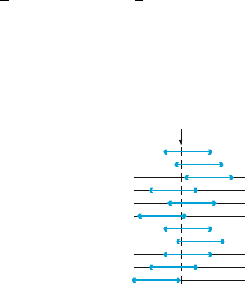
A correct interpretation of “95% confidence” relies on the long-run relative

frequency interpretation of probability: To say that an event A has probability .95 is

to say that if the experiment on which A is defined is performed over and over

again, in the long run A will occur 95% of the time. Suppose we obtain another

sample of typists’ preferred heights and compute another 95% interval. Then we

consider repeating this for a third sample, a fourth sample, and so on. Let A be the

event that

X  1 :96  s=

ﬃﬃﬃ

< m < X þ 1 :96  s=

ﬃﬃﬃ

. Since P(A) ¼ .95, in the long

run 95% of our computed CIs will contain m. This is illustrated in Figure 8.3, where

the vertical line cuts the measurement axis at the true (but unknown) value of m.

Notice that of the 11 intervals pictured, only intervals 3 and 11 fail to contain m.In

the long run, only 5% of the intervals so constructed would fail to contain m.

According to this interpretation, the confidence level 95% is not so much a

statement about any particular interval such as (79.3, 80.7), but pertains to what

would happen if a very large number of like intervals were to be constructed using

the same formula. Although this may seem unsatisfactory, the root of the difficulty

lies with our interp retation of probability—it applies to a long sequence of replica-

tions of an experiment rather than just a single replic ation. There is another

approach to the construc tion and interpretation of CIs that uses the notion of

subjective probability and Bayes’ theorem, as discu ssed in Sect ion 14.4. The

interval pres ented here (as well as each interval presented subsequently) is called

a “classical” CI because its interpretation rests on the classical notion of probability

(although the main ideas were developed as recently as the 1930s).

Other Levels of Conﬁdence

The confidence level of 95% was inherited from the probability .95 for the initial

inequalities in (8.2). If a confidence level of 99% is desired, the initial probability

of .95 must be replaced by .99, which necessitates changing the z critical value from

1.96 to 2.58. A 99% CI then resu lts from using 2.58 in place of 1.96 in the formula

for the 95% CI.

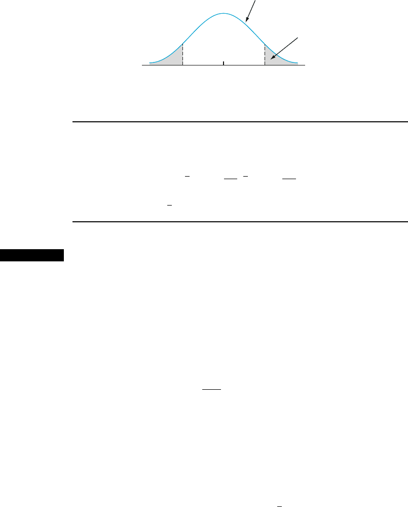
This suggests that any desired level of confidence can be achieved by

replacing 1.96 or 2.58 with the appropriate standard normal critical value. As

Figure 8.4 shows, a probability of 1  a is achieved by using z

a/2

in place of 1.96.

Interval

number

(1)

(2)

(3)

(4)

(5)

(6)

(7)

(8)

(9)

(10)

(11)

True value of m

Figure 8.3 Repeated construction of 95% CIs

386

CHAPTER 8 Statistical Intervals Based on a Single Sample

DEFINITION

A 100(1  a)% confidence interval for the mean m of a normal population

when the value of s is known is given by

x  z

a=2



ﬃﬃﬃ

;

x þ z

a=2



ﬃﬃﬃ



ð8:5Þ

or, equivalently, by

x  z

a=2

 s=

ﬃﬃﬃ

Example 8.3 A finite mathematics course has recently been changed, and the homework is now

done online via computer instead of from the textbook exercises. How can we see if

there has been improvement? Past experience suggests that the distribution of final

exam scores is normally distributed with mean 65 and standard deviation 13. It is

believed that the distribution is still normal with standard deviation 13, but the

mean has likely changed. A sample of 40 students has a mean final exam score of

70.7. Let’s calculate a confidence interval for the population mean using a confi-

dence level of 90%. This require s that 100(1  a) ¼ 90, from which a ¼ .10 and

a/2

¼ z

.05

¼ 1.645 (corresponding to a cumulative z-curve area of .9500).

The desired interval is then

70:7  1:645 

ﬃﬃﬃﬃﬃ

¼ 70:7  3:4 ¼ð67:3; 74:1Þ

With a reasonably high degree of confidence, we can say that 67.3 < m < 74.1.

Furthermore, we are confident that the population mean has improved over the

previous value of 65.

■

Conﬁdence Level, Precision, and Choice of Sample Size

Why settle for a confidence level of 95% when a level of 99% is achievable?

Because the price paid for the higher confidence level is a wider interval. The

95% interval extends 1:96  s=

ﬃﬃﬃ

to each side of

x, so the width of the interval is

2ð1:96Þs=

ﬃﬃﬃ

¼ 3:92  s=

ﬃﬃﬃ

. Similarly, the width of the 99% interval is

2ð2:58Þs=

ﬃﬃﬃ

¼ 5:16  s=

ﬃﬃﬃ

. That is, we have more confidence in the 99%

interval precisely because it is wider. The higher the desired degree of confidence,

the wider the resulting interval. In fact, the only 100% CI for m is (1, 1), which

is not terribly informative because, even before sampling, we knew that this

interval covers m.

z curve

1 − a

Shaded area = a /2

−z

a/2

Figure 8.4

(

-z



) ¼ 1a

8.1 Basic Properties of Conﬁdence Intervals 387