Devore J.L., Berk K.N. Modern Mathematical Statistics with Applications

Подождите немного. Документ загружается.

In the examples thus far, both steps 1 and 2 were carried out in an ad hoc manner

through intuition. For example, when the underlying population was assumed normal

with mean m and known s, we were led from

X to the standardized test statistic

Z ¼

X  m

ﬃﬃﬃ

For testing H

: m ¼ m

versus H

: m > m

, intuition then suggested rejecting H

when z was large. Finally, the critical value was determined by specifying the level

of significance a and using the fact that Z has a standard normal distribution when

is true. The reliability of the test in reaching a correct decision can be assessed

by studying type II error probabiliti es.

Issues to be considered in carrying out steps 1–3 encompass the following

questions:

1. What are the practical implications and consequence s of choosing a particular

level of significance once the other aspects of a test procedure have been

determined?

2. Does there exist a general principle, not dependent just on intuition, that can be

used to obtain best or good test procedures?

3. When two or more tests are appropriate in a given situation, how can the tests be

compared to decide which should be used?

4. If a test is derived under specific assumptions about the distribution or

population being sampled, how well will the test procedure work when the

assumptions are violated?

Statistical Versus Practical Signiﬁcance

Although the process of reaching a decision by using the methodology of classical

hypothesis testing involves selecting a level of significance and then rejecting or

not rejecting H

at that level, simply reporting the a used and the decisio n reached

conveys little of the information contained in the sample data. Especially when the

results of an experiment are to be communicated to a large audience, rejection of H

at level .05 will be much more convi ncing if the observed value of the test statistic

greatly exceeds the 5% critical value than if it barely exceeds that value. This is

Table 9.1 An illustration of the effect of sample size on P-values and b

nP-value when



= 101 b(101) for Level .01 Test

25 .3085 .9664

100 .1587 .9082

400 .0228 .6293

900 .0013 .2514

1600 .0000335 .0475

2500 .000000297 .0038

10,000 7.69  10

24

.0000

468

CHAPTER 9 Tests of Hypotheses Based on a Single Sample

precisely what led to the notion of P-value as a way of reporting significance

without imposing a particular a on others who might wish to draw their own

conclusions.

Even if a P-value is included in a summary of results, however, there may be

difficulty in interpreting this value and in making a decision. This is because a

small P-value, which would ordinarily indicate statistical significance in that it

would strongly suggest rejection of H

in favor of H

, may be the result of a large

sample size in combination with a departure from H

that has little pract ical

significance. In many experimental situations, only departures from H

of large

magnitude would be worthy of detection, whereas a small departure from H

would

have little practical significance.

Consider as an example testing H

: m ¼ 100 versus H

: m > 100 where m is

the mean of a normal population with s ¼ 10. Suppose a true value of m ¼ 101

would not represent a serious departure from H

in the sense that not rejecting H

when m ¼ 101 would be a relatively inexpensive error. For a reasonably large

sample size n, this m would lead to an

x value near 101, so we would not want this

sample evidence to argue strongly for rejecti on of H

when x ¼ 101 is observed.

For various sample sizes, Table 9.1 records both the P-value when

x ¼ 101 and also

the probability of not rejecting H

at level .01 when m ¼ 101.

The second column in Table 9.1 shows that even for moderately large sample

sizes, the P-value of

x ¼ 101 argues very strongly for rejection of H

, whe reas

the observed

x itself suggests that in practical terms the true value of m differs little

from the null value m

¼ 100. The third column points out that even when there is

little practical difference between the true m and the null value, for a fixed level of

significance a large sample size will almost always lead to rejection of the null

hypothesis at that level. To summarize, one must be especially careful in interpret-

ing evidence when the sam ple size is large, since any small departure from H

will

almost surely be detected by a test, yet such a departure may have little practical

significance.

Best Tests for Simple Hypotheses

The test procedures present ed thus far are (hopefully) intuitively reasonable, but

have not been shown to be best in any sense. How can an optimal test be obtained,

one for which the type II error probability is as small as possible, subject to

controlling the type I error probability at the desired level? Our starting point

here will be a rather unrealistic situation from a practical viewpoint: testing a

simple null hypothesis against a simple alternative hypothesis. A simple hypothesis

is one which, when true, completely specifies the distribution of the sample X

’s.

Suppose, for example, that the X

’s form a random sample from an exponential

distribution with parameter l. Then the hypothesis H: l ¼ 1 is simple, since when

H is true each X

has an exponential distribution with parameter l ¼ 1. We might

then consider H

: l ¼ 1 versus H

: l ¼ 2, both of which are simple hypotheses.

The hypothesis H: l  1 is not simple, because whe n H is true, the distribution of

each X

might be exponential with l ¼ 1 or with l ¼ .8 or .... Similarly, if the X

’s

constitute a random sample from a normal distribution with known s, then

H: m ¼ 100 is a simple hypothesis. But if the value of s is unknown, this hypothesis

is not simple because the distribution of each X

is then not completely specified; it

could be normal with m ¼ 100 and s ¼ 15 or normal with m ¼ 100 and s ¼ 12 or

9.5 Some Comments on Selecting a Test Procedure 469

normal with m ¼ 100 and any other positive value of s. For a hypothesis to be

simple, the value of every parameter in the pmf or pdf of the X

’s must be specified.

The next result was a milestone in the theory of hypothesis testing—a method

for constructing a best test for a simple null hypothesis versus a simple alternative

hypothesis. Let f(x

, ... , x

; y) be the joint pmf or pdf of the X

’s. Then our null

hypothesis will assert that y ¼ y

and the relevant alternative hypothesis will claim

that y ¼ y

. The result will carry over to the case of more than one parameter as

long as the value of each parameter is completely specified in both H

and H

THE

NEYMAN-

PEARSON

THEOREM

For testing a simple null hypothesis H

: y ¼ y

versus a simple alternative

hypothesis H

: y ¼ y

, let k be a positive fixed number and form the rejection

region



¼ðx

; ...; x

Þ:

f ð x

; ...; x

; y

f ð x

; ...; x

; y

 k



Thus R* is the set of all observations for which the likelihood ratio—ratio of

the alternative likelihood to the null likelihood—is at least k. The probability

of a type I error for the test with this rejection region is a* ¼ P[(X

, ..., X

)

∈ R* when y ¼ y

], whereas the type II error probability b* is the probability

that the X

’s lie in the complement of R* (in the “acc eptance” region) when

y ¼ y

Then for any other test procedure with type I error probability a

satisfying a  a*, the probability of a type II error must satisfy b  b*.

Thus the test with rejection region R* has the smallest type II error probabil-

ity among all tests for which the type I error probability is at most a *.

The choice of the constant k in the rejection region will determine the type I

error probability a*. In the continuous case, k can be selected to give one of the

traditional significance levels .05, .01, and so on, whereas in the discrete case

a* ¼ .057 or .039 may be as close as one can get to .05.

Example 9.20 Consider randomly selecting n ¼ 5 new vehicles of a certain type and determining

the number of major defects on each one. Letting X

denote the number of such

defects for the ith selected vehicle (i ¼ 1, ... ,5), suppos e that the X

’s form

a random sample from a Poisson distribution with parame ter l. Let’s find the

best test for testing H

: l ¼ 1 versus H

: l ¼ 2. The Poisson likelihood is

f ð x

;:::;x

; lÞ¼e

5l

=Px

!. Substituting first l ¼ 2, then l ¼ 1, and then

taking the ratio of these two likelihoods gives the rejection region



¼ðx

; ...; x

Þ : e

5

 k



Multiplying both sides of the inequality by e

and letting k

¼ ke

gives the

rejection region 2

 k

. Now take the natural logarithm of both sides and let

c ¼ ln(k

)/ln(2) to obtain the rejection region Sx

 c.

This latter rejection region is completely equi valent to R*: For any particular

value k there will be a corresponding value c, and vice versa. But it is much easier to

470 CHAPTER 9 Tests of Hypotheses Based on a Single Sample

express the rejection region in this latter form and then select c to obtain a desired

significance level than it is to determine an appropri ate value of k for the likelihood

ratio. In particular, T ¼ SX

has a Poisson distribution with parameter 5l (via a

moment generating function argument), so when H

is true T has a Poisson dis-

tribution with parameter 5. From the 5.0 column of our Poisson table (Table A.2),

the cumulative probabilities for the values 8 and 9 are .932 and .968, respectively.

Thus if we use c ¼ 9 in the rejection region,



¼ PðPoisson rv with parameter 5 is  9Þ¼1  :932 ¼ :068

Choosing instead c ¼ 10 gives a* ¼ .032. If we insist that the significance level be

at most .05, then the optimal rejection region is Sx

 10.

When H

is true, the test statistic has a Poisson distribution with parameter 10.

Thus



¼ PH

is not reject ed when H

is trueðÞ

¼ PðPoisson rv with parameter 10 is  9Þ¼:458

Obviously this type II error probability is quite large. This is because the sample

size n ¼ 5 is too small to allow for effective discrimination between l ¼ 1 and

l ¼ 2. For a sample size of 10, the Poisson table reveals that the best test havi ng

significance level at most .05 uses c ¼ 16, for which a* ¼ .049 (Poisson para-

meter ¼ 10) and b* ¼ .157 (Poisson parameter ¼ 20).

Finally, returning to a sample size of 5, c ¼ 10 implies that 10 ¼ ln(ke

)/ln(2),

from which k ¼ 2

 6.9. For the best test to have a significance level of at most

.05, the null hypothesis should be rejected only when the likelihood for the alternative

value of l is more than about 7 times what it is for the null value.

■

Example 9.21 Let X

, ... , X

be a random sample from a normal distribution with mean m and

variance 1 (the argument to be given will work for any other known value of s

Consider testing H

: m ¼ m

versus H

: m ¼ m

where m

> m

The likelihood ratio is



n=2

ð1=2ÞSðx

m



n=2

ð1=2ÞSðx

m

¼ e

m

ðn=2Þ m

m

ðÞ

¼ e

nðm

m

Þ=2

 e

ðm

m

ÞSx

The term in the first set of brackets is a numerical constant. Then m

 m

> 0

implies that the likelihood ratio will be at least k if and only if Sx

 k

, that is, if

and only if

x  k

, which means if and only if

z ¼

x  m

ﬃﬃﬃ

 c

If we now let c ¼ z

.01

¼ 2.33, this z test (one for which the test statistic has a

standard normal distribution when H

is true), will have minimum b among all tests

for which a  .01.

■

The key idea in these last two examples cannot be overemphasized: Write an

expression for the likelihood ratio, and then manipulate the inequality likelihood

ratio  k so it is equivalent to an inequality involving a test statistic whose distribution

when H

is true is known or can be derived. Then this known or derived distribution

9.5 Some Comments on Selecting a Test Procedure 471

can be used to obtain a test with the desired a. In the first example the distribution was

Poisson with parameter 5, and in the second it was the standard normal distribution.

Proof of the Neyman-Pearson Theorem: We shall consider the case in which the

’s have a discrete distribution, so that type I and type II error probabilities are

obtained by summation. In the continuou s case, integration replaces summation.

Then



¼fx

; ...; x

ðÞ: fx

; ...; x

; y

ðÞk  fx

; ...; x

; y

ðÞg



¼ P½ðX

; ...; X

Þ2R



when y ¼ y

¼



f ð x

; ...; x

; y



¼ P½ðX

; ...; X

Þ2R

0

when y ¼ y

¼

0

f ð x

; ...; x

; y

(b* is the sum over values in the complement of the rejection region). Suppose that

R is a rejection region different from R* whose type I error probability is at most a*;

that is,

a ¼ P½ðX

; ...; X

Þ2R when y ¼ y

¼

f ð x

; ...; x

; y

Þa



We then wish to show that b for this rejection region must be at least as large

as b*. Consider the difference

D ¼



½f ðx

; ...; x

; y

Þk  f ðx

; ...; x

; y

Þ



½f ðx

; ...; x

; y

Þk  f ðx

; ...; x

; y

Þ



½...þ



½...

R\R



½...þ

R\R



½...

()



½...

R\R



½...

This last dif ference is nonnegati ve (i.e.  0) because the term in the square brackets

is  0 for any set of x

’s in R* and is negative for any set of x

’s not in R*. It then

follows that

0 



f ð x

; ...; x

; y

Þk



f ð x

; ...; x

; y



f ð x

; ...; x

; y

Þþk

f ðx

; ...; x

; y

¼ð1  b



Þka



ð1  bÞþka

¼ b  b



 kða



 aÞb  b



ðsince a  a



implies that the term being subtracted is nonnegative Þ

Thus we have shown that b*  b as desired. ■

472 CHAPTER 9 Tests of Hypotheses Based on a Single Sample

Power and Uniformly Most Powerful Tests

The Neyman–Pearson theo rem can be restat ed in a slightly different way by

considering the power of a test, first introduced in Section 9.2.

DEFINITION

Let O

and O

be two disjoint sets of possible values of y, and consider testing

: y ∈ O

versus H

: y ∈ O

using a test with rejection region R. Then the

power function of the test, denoted by p( ) is the probability of rejecting H

considered as a function of y:

pðy

Þ¼P½ X

; :::; X

ðÞ2R when y ¼ y



Since we don’t want to reject the null hypothesis when y ∈ O

and do want to reject

it when y ∈ O

, we wish a test for which the power function is close to 0 whenever

is in O

and close to 1 whenever y

is in O

. The power is easily related to the

type I and type II error proba bilities:

pðy

Þ¼

Pðtype I error when y ¼ y

Þ¼aðy

Þ when y

2 O

1  Pðtype II error when y ¼ y

Þ¼1  bðy

Þ when y

2 O

(

Thus large power when y

∈ O

is equivalent to small b for such parameter values.

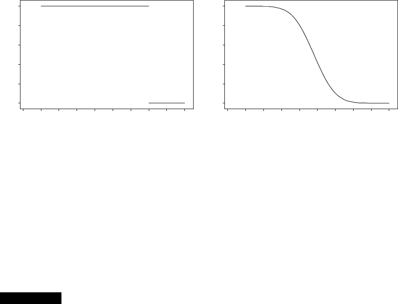
Example 9.22 The drying time (min) of a particular brand and type of paint on a test board under

controlled conditions is known to be normally distributed with m ¼ 75 and s ¼ 9.4. A

new additive has been developed for the purpose of improving drying time. Assume

that drying time with the additive is still normally distributed with the same standard

deviation, and consider testing H

: m  75 versus H

: m < 75 based on a sample of

size n ¼ 100. A test with significance level .01 rejects H

if z 2.33, where

z ¼ð

x  75Þ=ð9:4=

ﬃﬃﬃﬃﬃﬃﬃﬃ

100

Þ¼ðx  75Þ=:94. Manipulating the inequality in the rejec-

tion region to isolate

x gives the equivalent rejection region x  72:81. Thus the

power of the test when m ¼ 70 (a substantial departure from the null hypothesis) is

pð70Þ¼Pð

X  72:81 when m ¼ 70Þ¼F

72:81  70

9:4=

ﬃﬃﬃﬃﬃﬃﬃﬃ

100



¼ Fð2:99Þ¼:9986

so b ¼ .0014. It is easily verified that p(75) ¼ .01, the significance level. The

power when m ¼ 76 (a parameter value for which H

is true) is

pð76Þ¼Pð

X  72:81 when m ¼ 76Þ¼F

72:81  76

9:4=

ﬃﬃﬃﬃﬃﬃﬃﬃ

100



¼ Fð3:39Þ¼:0003

which is quite small as it should be. By repeating this calculation for various

other values of m we obtain the entire power function. A graph of the ideal

power function appears in Figure 9.10(a) and the actual power function is graphed

in Figure 9.10(b). The maximum power for m  75 (i.e. in O

)occursatm ¼ 75, on

the boundary between O

and O

. Because the power function is continuous, there are

values of m smaller than 75 for which the power is quite small. Even with a large

sample size, it is difficult to detect a very small departure from the null hypothesis.

9.5 Some Comments on Selecting a Test Procedure 473

The Neyman–Pearson theorem says that when O

consists of a single value

and O

also consists of a single value y

, the rejection region R* specifies a test

for which the power p(y

) at the alternative value y

(which is just 1  b )is

maximized subject to p(y

)  a for some specified value of a . That is, R* specifies

a most powerful test subject to the restriction on the power when the null hypothesis

is true.

What about best tests when at least one of the two hypothese s is composite,

that is, O

or O

(or both) consist of more than a single value?

Example 9.23

(Example 9.20

continued)

Consider again a random sample of size n ¼ 5 from a Poisson distribution, and

suppose we now wish to test H

: l  1 versus H

: l > 1. Both of these hypotheses

are composite. Arguing as in Example 9.20, for any value l

exceeding 1, a most

powerful test of H

: l ¼ 1 versus H

: l ¼ l

with significance level (power when

l ¼ 1) .032 rejects the null hypothesis when Sx

 10. Furthermore, it is easily

verified that the power of this test at l

is smaller than .032 if l

< 1. Thus the test

that rejects H

: l  1 in favor of H

: l > 1 when Sx

 10 has maximum power

for any l

> 1 subject to the condition that p(l

)  .032. This test is uniformly most

powerful.

■

More generally, a uniformly most powerful (UMP) level a test is one for

which p(y

) is maximized for any y ∈ O

subject to p(y

)  a for any y

∈ O

Unfortunately UMP tests are fairly rare, especially in commonly encountered

situations when H

and H

are assertions about a single parameter y

whereas the

distribution of the X

’s involves not only y

but also at least one other “nuisance

parameter”. For example, when the population distribution is normal with values of

both m and s unknown, s is a nuisance parameter when testing H

: m ¼ m

versus

: m 6¼ m

. Be careful here—the null hypothesis is not simple because O

consists

of all pairs (m, s) for which m ¼ m

and s > 0, and there is certainly more than one

such pair. In this situation, the one-sample t test is not UMP.

ideal actual

0.0

68 69 70 71 72 73 74 75 76 77

0.2

0.4

0.6

IDEAL POWER

MEAN

68 69 70 71 72 73 74 75 76 77

MEAN

0.8

1.0

0.0

0.2

0.4

0.6

POWER

0.8

1.0

Figure 9.10 Graphs of power functions for Example 9.22 ■

474

CHAPTER 9 Tests of Hypotheses Based on a Single Sample

However, suppose we restrict attention to unbiased tests, those for which the

smallest value of p(y

)fory

∈ O

is at least as large as the largest value of p(y

)for

∈ O

. Unbiasedness simply says that we are at least as likely to reject the null

hypothesis when H

is false as we are to reject it when H

is true. The test proposed in

Example 9.22 involving paint drying times is unbiased because, as Figure 9.10(b)

shows, the power function at or to the right of 75 is smaller than it is to the left of 75.

It can be shown that the one-sample t test is UMP unbiased; that is, it is uniformly

most powerful among all tests that are unbiased. Several other commonly used tests

also have this property. Please consult one of the chapter references for more details.

Likelihood Ratio Tests

The likelihood ratio (LR) principle is the most frequently used method for finding an

appropriate test statistic in a new situation. As before, denote the joint pmf or pdf of

, ... , X

by f(x

, ... , x

; y). In the case of a random sample, it will be a product

f(x

;y)







f(x

;y). When the x

’s are the actual observations and f(x

, ... , x

;y)is

regarded as a function of y,itiscalledthelikelihood function. Again consider

testing H

: y ∈ O

versus H

: y ∈ O

,whereO

and O

are disjoint sets, and

let O ¼ O

[ O

. In the Neyman–Pearson theorem, we focused on the ratio of the

likelihood when y ∈ O

to the likelihood when y ∈ O

, rejecting H

when the value of

the ratio was “sufficiently large”. Now we consider the ratio of the likelihood when

y ∈ O

to the likelihood when y ∈ O. A very small value of this ratio argues against

the null hypothesis, since a small value arises when the data is much more consistent

with the alternative hypothesis than with the null hypothesis. More formally,

1. Find the largest value of the likelihood for any y ∈ O

by finding the maximum

likelihood estimate of y within O

and substituting this mle into the

likelihood function to obta in Lð

Þ.

2. Find the largest value of the likelihoo d for any y ∈ O by finding the maximum

likelihood estimate of y within O and substituting this mle into the likelihood

function to obtain Lð

OÞ. Because O

is a subset of O, this likelihood Lð

OÞ can’t

be any smaller than the likelihood Lð

Þ obtained in the first step, and will be

much larger when the data is much more consistent with H

than with H

3. Form the likelihood ratio Lð

Þ=Lð

OÞand reject the null hypothesis in favor

of the alternative when this ratio is  k. The critical value k is chosen to give a

test with the desired significance level. In practice, the inequality Lð

Þ=Lð

OÞk

is often re-expressed in terms of a more convenient statistic (such as the sum

of the observations) whose distribution is known or can be derived.

The above prescription remains valid if the single parameter y is replaced by

several parameters y

, ... , y

. The mle’s of all parameters must be obtained in

both steps 1 and 2 and substituted back into the likelihood function.

Example 9.24 Consider a random sample from a normal distribution with the values of both

parameters unknown. We wish to test H

: m ¼ m

versus H

: m 6¼ m

. Here O

consists of all values of m and s

for which 1 < m < 1 and s

> 0, and the

likelihood function is

2ps



n=2

1=ð2s

ðx

mÞ

9.5 Some Comments on Selecting a Test Procedure 475

In Section 7.2 we obtained the mle’s as

m ¼ x;

ðx

 xÞ

=n: Substituting

these estimates back into the likelihood function gives

Lð

OÞ¼

ðx

 xÞ



n=2

n=2

Within O

, m in the foregoing likelihood is replaced by m

, so that only s

must be

estimated. It is easily verified that the mle is

ðx

 m

=n: Substitution of

this estimate in the likelihood function yields

Lð

Þ¼

ðx

 m



n=2

n=2

Thus we reject H

in favor of H

when

Lð

OÞ

ðx

 xÞ

ðx

 m

n=2

 k

Raising both sides of this inequality to the power 2/n, we reject H

whenever

ðx

 xÞ

ðx

 m

 k

2=n

¼ k

This is intuitively quite reasonable: the value m

is implausible for m if the sum of

squared deviations about the sample mean is much smaller than the sum of squared

deviations about m

. The denominator of this latter ratio can be expressed as

½ðx

 xÞþðx  m

Þ

ðx

 xÞ

þ 2

ðx  m

Þðx

 xÞþnðx  m

The middle (i.e., cross-product) term in this expression is 0, because the constant

x  m

can be moved outside the summation, and then the sum of deviations from

the sample mean is 0. Thus we should reject H

when

ðx

 xÞ

ðx

 xÞ

þ nðx  m

1 þ nð

x  m

ðx

 xÞ

 k

This latter ratio will be small when the second term in the denominator is large, so

the condition for reject ion becomes

nðx  m

ðx

 xÞ

 k

Dividing both sides by n  1 and taking square roots gives the rejection region

either

x  m

ﬃﬃﬃ

 c or

x  m

ﬃﬃﬃ

c

If we now let c ¼ t

a=2;n1

, we have exactly the two-tailed one-sample t test. The

bottom line is that when testing H

: m ¼ m

against the two-sided (6¼) alternative,

the one-sample t test is the likelihood ratio test. This is also true of the upper-tailed

version of the t test when the alternative is H

: m > m

and of the lower-tailed test

when the alternative is H

: m < m

. We could trace back through the argument to

recover the critical constant k from c, but there is no point in doing this; the

rejection region in terms of t is much more convenient than the rejection region

in terms of the likelihood ratio.

■

476 CHAPTER 9 Tests of Hypotheses Based on a Single Sample

A number of tests discussed subsequently, including the “pooled” t test from

the next chapter and various tests from ANOVA (the analysis of variance) and

regression analysis, can be derived by the likelihood ratio principle. Rather fre-

quently the inequality for the rejection region of a likelihood ratio test cannot be

manipulated to express the test procedure in terms of a simple statistic whose

distribution can be ascertained. The following large-sample result, valid under

fairly general conditions, can then be used: If the sample size n is suffic iently

large, then the statistic 2[ln(likelihood ratio)] has approximately a chi-squared

distribution with n degrees of freedom, where n is the difference between the

number of “freely varying” parameters in O and the number of such parameters

in O

For example, if the distribution sampled is bivariate normal with the 5 para-

meters m

, m

, and r and the null hypothesis asserts that m

¼ m

and

¼ s

, then n ¼ 5  3 ¼ 2. By definition Lð

Þ=Lð

OÞ1, and the likelihood

ratio test rejects H

when this likelihood ratio is much less than 1. This is equivalent

to rejecting when the logarithm of the likelihood ratio is quite negative, that is,

when ln(LR) is quite posi tive. The large- sample version of the test is thus upper-

tailed: H

should be rejected if 2ln(likelihood ratio)  w

a;n

(an upper-tail critical

value extracted from Table A.6).

Example 9.25 Suppose a scientist makes n measurements of some physical characteristic, such as

the specific gravity of a liquid. Let X

, ... , X

denote the resulting measurement

errors. Assume that these X

’s are independent and identically distributed according

to the double exponential (Laplace) distribution: f ðxÞ¼:5e

 xyjj

for 1<x <1:

This pdf is symmetric about y with somewhat heavier tails than the normal pdf.

If y ¼ 0 then the measurements are unbiased, so it is natural to test H

: y ¼ 0 versus

: y 6¼ 0. Here n ¼ 1  0 ¼ 1. The likelihood is

LðyÞ¼ð:5Þ

S x

y

Because of the minus sign preceding the summation, the likelihood is maximized

when

 yj is minimized. The absolute value function is not differentiable,

and therefore dif ferential calculus cannot be used. Instead, consider for a moment

the case n ¼ 5 and let y

, ..., y

denote the values of the x

’s ordered from smallest

to largest—so the y

’s are the observed values of the order statistics. For example, a

random sample of size five from the Laplace distribution with y ¼ 0is.24998,

.75446, .19053, 1.16237, .83229, so (y

, ..., y

) ¼ (.24998, .19053, .75446,

.83229, 1.16237) . Then

 y

 yj¼

þ y

 5yy< y

y

þ y

 3y y

 y < y

y

 y

þ y

 y y

 y < y

y

 y

þ y

þ y y

 y < y

y

 y

þ y

þ 3y y

 y < y

y

 y

þ 5yy y

The graph of this expression as a function of y appears in Figure 9.11, from which it

is apparent that the minimum occurs at y

x ¼ :75446, the sample median. The

situation is similar whenever n is odd. When n is even, the function achieves its

minimum for any y between y

n/2

and y

(n/2)+1

; one such y is ðy

n=2

þ y

ðn=2Þþ1

Þ=2 ¼

In summary, the mle of y is the sample median.

9.5 Some Comments on Selecting a Test Procedure 477