Dorst L., Fontijne D., Mann S. Geometric Algebra for Computer Science. An Object Oriented Approach to Geometry

Подождите немного. Документ загружается.

292 THE HOMOGENEOUS MODEL CHAPTER 11

11.7 INCIDENCE RELATIONSHIPS

The ﬂats we have introduced can be combined. The outcome of spanning operations,

duality, and incidence operations on ﬂats are again ﬂats. They form a complete system of

computing with such relationships between offset subspaces. This could of course only be

achieved by encoding both the proper ﬂats and the improper ﬂats. Two planes now always

have a line in common, even when they are parallel (in which case it is an improper line

at inﬁnity).

These geometrical properties are reﬂected in our algebra by closure under ∧,

∗

, and ∩

(since the

meet is the dual of the outer product of the duals, the third follows automatically

from the others). In particular, whatever computation we perform, we will always obtain

an element of the algebra. There is therefore no need for exceptional treatment of lines,

points, directions, and so on; we can always compute on, regardless of the type of the

outcome. Only at the ver y end of our computations, when we need to render the results,

we may need to test for the type of element that is the ﬁnal outcome, and compute its

parameters.

11.7.1 EXAMPLES OF INCIDENCE COMPUTATIONS

We give some examples of incidences in the homogeneous model, expanding the natural

form A ∩B = B

∗

A of the meet in Chapter 5 down to the consequences for the Euclidean

parameters of the ﬂats in the base space. The purpose of this is not to show you how to

do such computations, for you would never do them in real life. Your geometric algebra

software will automatically take care of computation and interpretation in a structural

manner. But to learn to rely on that, you need to see the correspondence to the classical

approach at least once. This permits us to point out the differences, and demonstrate how

the uniﬁcation of the structure can simplify the ﬂow of your code.

Two Lines in a Plane

When we have two lines in the same plane I through the origin in R

,sayL = e

u + U

and M = e

v + V, their meet at a point can be computed. For this we need their join.

Assuming ﬁrst that the lines are in general position in the plane I, the

join is the com-

mon plane representative e

I in the homogeneous representation space R

n+1

. Since both

arguments of the

meet are of the same type, it is convenient to use the dual computation

L ∩ M = (M

∗

∧ L

∗

)

−∗

. We rewrite a dual in terms of the Euclidean dual:

∗

= (e

u + U) I

−1

= −u

夹

+ U

夹

−1

You should realize that in the plane considered, u

夹

isavectorandU

夹

is a scalar. Their

commutative properties then enable a fairly quick simpliﬁcation of results:

SECTION 11.7 INCIDENCE RELATIONSHIPS 293

L ∩ M =



(−v

夹

+ V

夹

−1

) ∧ (−u

夹

+ U

夹

−1

)



−∗

= (v

夹

∧ u

夹

)

−∗

+ (V

夹

−1

)

−∗

− (U

夹

−1

)

−∗

= e

夹

∧ u

夹

)

−夹

+ V

夹

u − U

夹

= e

(u ∧ v)

夹

+ V

夹

u − U

夹

v. (11.8)

(For the ﬁnal step, we used (v

夹

∧ u

夹

)

−夹

= v

夹

·u = u·v

夹

= (u ∧ v)

夹

. ) That is the result of

the

meet with this join as the plane of the lines. Depending on whether (u ∧ v)

夹

is zero

or not, we have two interpretations: the lines intersect in a ﬁnite point or in an inﬁnite

point. Therefore, a single computation in the homogeneous model

n+1

captures several

cases that are different in

. We spell them out to show that they correspond to some

familiar expressions.

•

Finite Intersect ion Point.If(u ∧ v)

夹

= 0, we can write the result of (11.8) as a

weighted point in its homogeneous representation:

L ∩ M = (u ∧ v)

夹



u ∧ v

u +

v ∧ u



This shows that the result is indeed a point, at the location

u∧v

u +

v∧u

v, and

withaweight(u ∧ v)

夹

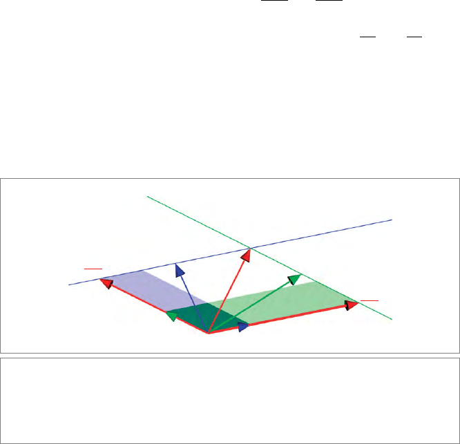
. The correctness of the location is illustrated in Figure 11.5.

We already met the geometry of this construction in Section 2.7.2, when we ﬁrst

encountered Cramer’s rule as a ratio of planar elements. The solution then was

rather ad hoc; we now see that it is simply a special case of the

meet operation.

Theweightofthe

meet, (u ∧ v)

夹

, is an interesting feature of the computation.

If we take u and v to be unit vectors (so that the lines L and M are normalized

V = q∧v

U = p∧u

u∧v

q∧v

u∧v

p∧u

v∧u

Figure 11.5: The intersection of two offset lines L and M to produce a point x. Their meet

tells us that the point x can be reached by translating e

over a multiple of u and a multiple of

v. We show graphically why the coefﬁcient for v is the ratio of the moment U of the line L and

the bivector of directions u ∧ v: the stretch factor of the vector v is the same as that of the

bivector u ∧ v to make U (taking reshapability into account).

294 THE HOMOGENEOUS MODEL CHAPTER 11

in this sense), this weight attributes a sign to the meet enabling us to know how

L and M intersect: positive when v points counterclockwise of u (in a plane w ith a

counterclockwise orientation), negative in the other direction. Moreover, the weight

is an intersection st rength that can be interpreted as a numerical stability of the

intersection; when the lines intersect perpendicularly it is strongest, and when they

are almost parallel the weig ht becomes very small (and if the lines would be noisy

data, their intersection would indeed get rather unlocalized).

•

Two Parallel Lines. When the weight (u ∧ v)

夹

equals zero, the lines are parallel.

Now the result of the

meet in (11.8) can be simpliﬁed to

L ∩ M = V

夹

u − U

夹

Since V

夹

and U

夹

are scalars, this is a multiple of the common direction u

(or v), so the lines now meet in a weighted improper point, although you

may prefer to say that they have a common direction. It is accompanied by a

weight, obviously proportional to the weight of the lines L and M, but also to

their relative position. If we take the lines to be unit lines (in the sense that u

and v are unit vectors), the dual moments are simply their oriented distances

to the origin, and the result simpliﬁes to (δ

−δ

) u.Sotwo parallel unit lines

intersect in a p oint at inﬁnit y weighted by their distance. This is an interestingly

compact quantitative combination of both their commonality (their direction)

and their difference (their distance).

•

Two Coincident Lines. When the lines are not only parallel, but have distance zero,

the result of the

meet computation above is zero. As we noted in Chapter 5, this

indicates that we have reached a case in which we have the wrong

join to compute

the actual

meet (which should never be zero). Indeed, when the lines coincide, the

situation is rather trivial: their

join is the line, and so is their meet.

If the

meet computations above intimidated you, please realize that you don’t have to do

such computations by hand; the

meet operation will just give the right answer. It switches

cases automatically depending on the relative geometry of its input arguments.

But it is good to realize that the difference between the ﬁrst two conﬁgurations (general

or par allel) is actually not even a case switch for the

meet, since the join does not change.

The conﬁgurations merely appear as different cases if we need to interpret ﬁnite points

differently from inﬁnite points (for instance, to draw them using their parameters). That

happens only at the end of a chain of computations; if (11.8) was an intermediate result,

you could just compute on without splitting the data ﬂow of the program.

So in practice, you do not need to do such computations before you can write code. We

have only performed them here in detail to comment on the type of result, which is typi-

cal: coordinate-free, weighted, and merging separate geometrical cases. In your code, use

∗

L if you know that M and L are guaranteed not to be degener ate; if they may be, use

an algorithmic implementation of the

meet operation L ∩ M. The latter is much more

expensive, as we will ﬁnd in Section 21.7, and therefore to be avoided.

SECTION 11.7 INCIDENCE RELATIONSHIPS 295

Two Skew Lines in Space

When two lines L = p ∧ u = e

u + U and M = q ∧ v = e

v + V are in general position

in a 3-D space with pseudoscalar I

, their join in the homogeneous representation space

is of course the pseudoscalar e

. The technique for the computation of their meet is

similar to the simpler case above (alternatively, you can use the derivation of structural

exercise 11). The result now is

L ∩ M =



U ∧ v + u ∧ V



夹



(p − q) ∧ u ∧ v



夹



d (u ∧ v)



夹

(11.9)

which is a scalar containing both the directional dissimilarity (in terms of the sine of

the angle between u and v) and the locational dissimilarity (since it is proportional to

their weighted distance, which is the oriented length of their separation vector

d ≡



(p −q) ∧u ∧v



/(u ∧v) ). This is illustrated in Figure 11.6. In this case, you can only

retrieve the distance between the lines from the

meet when you know the meet of their

directions (u ∧ v)

∗

When the

meet computed in this manner becomes zero, it denotes the need for a new join

to compute the true meet. The algebr aic form of the meet shows that this can happen

in one of two ways: the factor (u ∧ v) can become zero, which means that the lines are

v∧p∧ u

u∧q∧v

Figure 11.6: The meet of two skew lines L = (e

+ p) ∧ u and M = (e

+ q) ∧ v in their

common space equals ((p − q) ∧ u ∧ v)

夹

, which can be interpreted as the difference of two

oriented volumes. You can perform a rejection to display the separation vector d, perpendicular

to u ∧ v, reexpressing the

meet as (d (u ∧ v))

夹

296 THE HOMOGENEOUS MODEL CHAPTER 11

parallel, or d can become zero, which means that the lines intersect. Geometrically, either

case implies that the lines have become coplanar; then the

join is no longer the space

, but their common plane, and the meet reduces essentially to the previous case.

11.7.2 RELATIVE ORIENTATION

When a meet of two elements A and B is scalar, it can be interpreted as a relative orienta-

tion with numerical signiﬁcance. We announced this when treating the

meet of subspaces

through the origin in Chapter 5. In terms of modeling, we were then using the vector space

model. The examples given there can now be generalized to offset ﬂats by employing the

homogeneous model.

If the

meet of A and B is scalar, then the elements A and B should be complementary

within the

join, since (5.4) states that the grades are related as m = a + b − j, so that

m = 0 implies a = j − b. We can then replace the contraction in the computation of the

meet by a scalar product, and use its symmetry to rewrite it to a proper dual relative to

the

join:

A ∩ B = (B

∗

)A = (B

∗

) ∗ A = A ∗ (B

∗

) = A(B

∗

) = (A ∧ B)

∗

Therefore the

meet in this scalar case is just the oriented volume measure of A and B (in

that order, and relative to the chosen orientation of the pseudoscalar for the subspace J

that determines the duality). We treat the most common case in 3-D Euclidean geometry

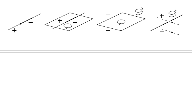
with a right-handed pseudoscalar. These are illust rated in Figure 11.7.

•

Two Points on a Line. In the homogeneous model, a line L is represented by a

2-blade. Introduce the pseudoscalar I

of this 2-blade. Now we can compute the

meet of two points p and q on this line L as

p ∩ q = (p ∧ q)

∗

(a) (b) (c) (d)

Figure 11.7: The relative orientation of oriented ﬂats: (a) the sides of a (unit) point on an

oriented line, (b) the sides of an oriented line in an oriented plane, (c) the sides of an oriented

plane in an oriented space, and (d) the sides of an oriented line in an oriented space. In (d),

the probes are oriented lines; in the other examples they are positively weighted points. The

right-handed corkscrews in (c) and (d) denote the orientation of the 3-D pseudoscalar.

SECTION 11.7 INCIDENCE RELATIONSHIPS 297

This is indeed a scalar and it changes sign as p and q change their order on the line L.

It does so continuously, being zero when p coincides with q (see Figure 11.7(a)). If

we use identical weighted points (for which e

−1

·p = e

−1

·q), the weight of the meet

is proportional to the oriented length of the line segment from p to q; in particular,

relativetoa

join of weight 1, and using its orientation as standard, one has p ∩ q =

(p ∧ q)

∗

= ±(q − p).

That is useful for comparing ratios along the same line. Unfortunately, the actual

proportionality constant is u



+ d

) (compute this in structural exercise 10),

which is different for almost all lines. Therefore, lengths of segments on different

lines cannot directly be compared in this manner; you would need to revert to

the vector space submodel or upgrade to the conformal model. The homogeneous

model is poorly suited for metrical computations.

•

A Point and a Line in Their Plane.Apointp and a line L = q ∧r also have comple-

mentar y grades in their plane, so we can determine their relative orientation as

p ∩ L = (p ∧ L)

∗

= (p ∧ q ∧ r)

∗

Taking the sign of this as the relative orientation, the positive side of the line L is such

that the orientation of p, q, and r is the same as that imposed on the plane by the

join. For a plane oriented in the customary counterclockwise fashion, the positive

side of L is therefore left of q∧r (see Figure 11.7(b)). In a plane with counterclockwise

orientation (what mathematicians think of as positive), the positive side of the line

is on your left when you look along its direction (as you can show by rewriting the

line to L = q ∧ (r − q) = q ∧ v ).

Theweightofthe

meet is proportional to the area of the triangle formed by p, q,

and r (by a factor that depends on q and r). As p varies from the left of the line to the

right, this changes smoothly from positive to negative, with zero when p is on the

line (which signals that we should change the

join to compute the actual meet). If

we keep the line ﬁxed in its parameters (i.e., keep q and r ﬁxed), then the value of the

meet is proportional to the (oriented) perp endicular distance of the point p to the

line L. The proportionality factor depends on the location of the plane relative to

the origin, but within the plane the measure is usable as a relative oriented distance

of points to the line.

•

A Point and a Plane in Space. Similarly, a point p can be on different sides of a

plane Π=q ∧ r ∧ s in space. The positive side of Π is where sign((p ∧ Π)

∗

) is pos-

itive, which is the side where the volume p ∧ q ∧ r ∧ s has the same orientation as

the volume measure assigned to the space. Usually one would take the right-handed

pseudoscalar e

∧ e

for that, which is equivalent to the orientation of the

tetrahedron formed by the points e

, e

+ e

, e

+ e

, e

+ e

(in that order!). The

volume measure of p ∧Π determines the quantitative aspects in a smoothly varying

manner, with zero occurring only if p is on the plane Π (see Figure 11.7(c)). For a

298 THE HOMOGENEOUS MODEL CHAPTER 11

right-handed space, orient the ﬁngers of your right hand with the plane, then your

thumb points away from the positive side. If we had deﬁned the relative orienta-

tion as the sign of (Π ∧ p)

∗

, we would get the opposite answer, for this meet is not

symmetric in its arguments; see Section 5.6.)

Numerically, the value of the

meet is proportional to the (oriented) perp endicular

distance of the point p to the plane Π.

•

Two Skew Lines in Space. It is somewhat harder to imagine that two oriented lines

L and M in space also have a relative orientation. This implies that there is a positive

side and a negative side to line L in space, though not for points as probes (so these

sides are hard to color), but for lines like M.

Once you realize it can be done, this is of course simple. If the lines are given though

points on them such as L = p ∧ q and M = r ∧ s, then the positive side is the one

where L ∧M = p ∧q ∧r ∧s has the same orientation as the pseudoscalar of the space.

This is illustrated in Figure 11.7(d), which shows some of the oriented line probes.

Theweightofthe

meet is now proportional to the (oriented) perpendicular dis-

tance between the two lines, weighted by the sine of the angle between their relative

directions.

A standard example would be the line L = e

∧ e

, with M = (e

+ e

) ∧ e

being

positive relative to it in right-handed space. In this case, L ∩M = (e

∧ e

)

∗

=+1, so this is positive. As an easy way to see the sign, view L as a rotation axis;

grab it with your right hand (!) and if M points similar to your ﬁngers, it is positive

relative to L. Note that the order does not matter: when L is positive relative to M,

then M is positive relative to L, for this

meet is symmetric in its arguments.

This relative orientation measure on lines can be used to determine whether a ray

M passes inside a triangle described by three consistently oriented boundary carrier

lines L

, L

: all signs of relative orientations with M should be equal.

11.7.3 RELATIVE LENGTHS: DISTANCE RATIO AND

CROSS RATIO

We have seen several computable measures that are proportional to Euclidean quantities

in which we are interested. They are accompanied by extra factors that make them unin-

terpretable by themselves. The giveaway is often the occurrence of e

or e

−1

—they should

never be present in a geometrical result, for they are only accidental elements of the repre-

sentation, not of reality. True, e

represents the point at the origin, but even that is really

arbitrary; since we allow translations in our geometry, we can move it anywhere. Yet it

is possible to perform computations that have an objective meaning in the base space.

We show what kind of length measurements are independent of the representation, and

under what conditions.

Consider three colinear points P, Q, R. We like to keep the representation as general

as possible, and do not even demand normalization of their representations. We denote

SECTION 11.7 INCIDENCE RELATIONSHIPS 299

p = p

+ p), and so on. A two-point combination (as occurs for instance in a meet)

depends on the scaling factors of the representation:

p ∧ q = p



∧ (p − q) + p ∧ q



= p

d (p − q),

where d = e

+ (p ∧ q)/(p − q) is the support point of the common line. Because of

the colinearity of the points, that support point can be factored out of other two-point

combinations as well, so, for instance,

q ∧ r = q

d (q − r).

When we take the ratio of these quantities, d cancels out, and the ratio of two bivectors

from

n+1

becomes the ratio of two vectors of R

afﬁne distance ratio :

p ∧ q

q ∧ r

p − q

q − r

. (11.10)

This is a scalar, since (p − q) and (q − r) are proportional vectors for the colinear points

p, q, and r.

For identically normalized points (so that p

= r

), this simpliﬁes to being the ratio

of oriented distances along a line. Only for transformations that do not change the

normalization of points is this a meaningful, invariant quantity that does not change

with the transformation. We are therefore interested in this class of transformations. In

Section 11.8.8 we show that they are precisely the afﬁne transformations of

. These

encompass all Euclidean transformations, notably the rigid body motions in the base

space

. We call the quantity (p ∧ q)/(q ∧ r) the afﬁne distance ratio to remind us that it

is an afﬁne invariant of the points p, q, and r.

The distance ratio would be invariant under an arbitrary linear transformations of

n+1

if it had not involved the normalization constants p

and r

at all. But we can simply

eliminate those by taking a similar ratio of p and r with another point s (also on the same

line), and then cancel all normalization factors by taking the ratio of two ratios. This is

called the (projective) cross ratio:



p ∧ q

q ∧ r



r ∧ s

s ∧ p





p − q

q − r



r − s

s − p



See Figure 11.8. This combination of four oriented distances of points along the same line

is not changed by any linear transformation of the homogeneous representation space.

Such arbitrary transformations in the homogeneous representation space

n+1

repre-

sent precisely the projective transformations of the base space

(often called colineations

or homographies). Projective transformations can affect distances and even the order of

points along a line severely, so it was quite a discovery (independently by Chasles and by

obius in the 1850s) that an invariant quantity could nevertheless be found. We discuss

projective transformations in Section 11.8.9.

300 THE HOMOGENEOUS MODEL CHAPTER 11

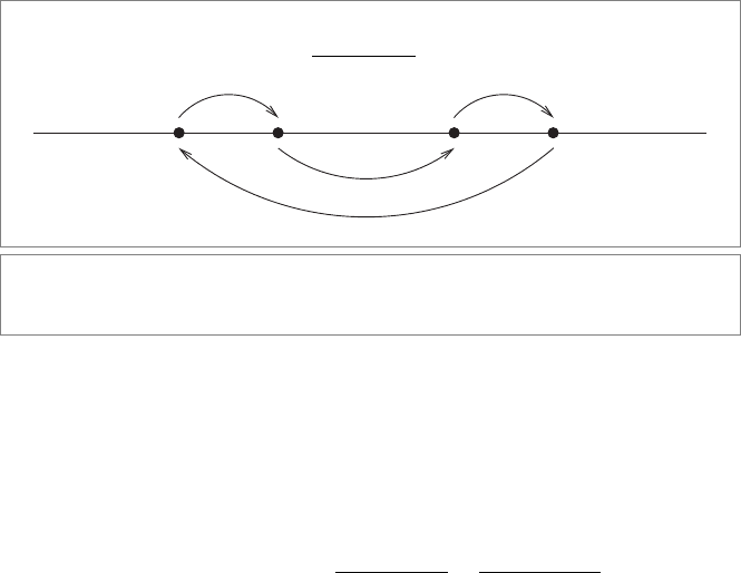
(p ∧ q) (r ∧ s)

(q ∧ r) (s ∧ p)

pq r s

Figure11.8: The combinations of four points taken in the cross ratio. The directed arcs above

the line go into the numerator, the directed arcs below the line into the denominator.

Note the particularly simple form the cross r atio takes in the embedding of the homo-

geneous model in geometr ic algebra, where the ratio of bivectors of

n+1

or vectors of

is well-deﬁned so that there is no need to ﬁrst reduce the factors to scalars (which is

necessarily the classical approach). Because of the commutation properties of all elements

involved, we can also rewrite the cross ratio to a single fraction:

projective cross ratio :

(p ∧ q)(r ∧ s)

(q ∧ r)(s ∧ p)

(p − q)(r − s)

(q − r)(s − p)

. (11.11)

Symmetry properties of the cross ratio follow from the antisymmetry of the cross product

of points (left of the equality), or the subtraction of vectors (right of the equality); see also

structural exercise 18.

This cross ratio of points on a common line can be extended simply to a cross ratio for

lines passing though a common point and lying in a common plane. One usually does so

by creating four points from those lines by intersecting the lines with an arbitrary ﬁfth

line, not through the common point, and using the resulting four points in a cross ratio

on that line. We can prove the correctness of this simply, as soon as we realize that we are

actually taking a cross ratio of areas rather than lines (just as the construction above is a

cross ratio of distances rather than points).

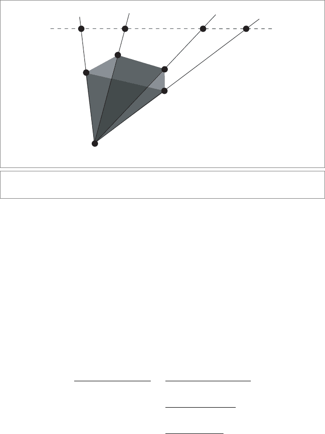
As depicted in Figure 11.9, we take a reference point x and four arbitrary points p, q, r,

s, and the four triangles determined by x and two of the other points. The area of the

triangle formed by x, p, q is proportional to the weight of x ∧p ∧q. To show the invariance

of the cross ratios, we rewrite them to the cross ratios of points on the arbitrary line L.

This requires deﬁning points p



and q



on that line, lying on the same rays from x as p and

q do. It changes each area measure, for

x ∧ p ∧ q = x ∧ (p − x) ∧ (q − x)

= x ∧ (p − x) ∧ (q − x)

SECTION 11.7 INCIDENCE RELATIONSHIPS 301

p⬘

q⬘

r⬘

s⬘

Figure 11.9: The combinations of four lines (actually, areas) taken in the cross ratio.

= x ∧



(p − x)



∧



(q − x)



/(p

)

= x ∧ (p



− x) ∧ (q



− x)/( p

)

= x ∧ p



∧ q



/(p

When we take the cross ratio of the four areas, these radial rescaling constants will cancel.

We have one more trick to play to get back to the cross ratio for lengths: recognizing that

all area elements can be written as multiples of x ∧L, we deﬁne the support point d of the

line L relative to x through the demand dL= x ∧ L. Then all areas are expressed in terms

of geometric products, and the common point support cancels in the ratio:

(x ∧ p ∧ q)(x ∧ r ∧ s)

(x ∧ q ∧ r)(x ∧ s ∧ p)

(x ∧ p



∧ q



)(x ∧ r



∧ s



)

(x ∧ q



∧ r



)(x ∧ s



∧ p



)

d (p



∧ q



) d (r



∧ s



)

d (q



∧ r



) d (s



∧ p



)



∧ q



)(r



∧ s



)



∧ r



)(s



∧ p



)

Since the ﬁnal result is invariant under projective transformations, the original area cross

ratio is invariant as well. Using the same principles, you can deﬁne an invariant cross ratio

of volumes containing a common line in 3-D, and corresponding quantities in higher-

dimensional spaces.