Dorst L., Fontijne D., Mann S. Geometric Algebra for Computer Science. An Object Oriented Approach to Geometry

Подождите немного. Документ загружается.

322 THE HOMOGENEOUS MODEL CHAPTER 11

is equivalent in performance to:

g_normalizedPoints[idx] = g_normalizedPoints[g_dragPoint] + T;

but it is more generic since it conforms to the general pattern. Geometric algebra has

enough structure to permit automated generation of implementations. Having such a

code generator permits you to introduce small optimizations like the normalized points

very easily. We discuss these techniques in Part III.

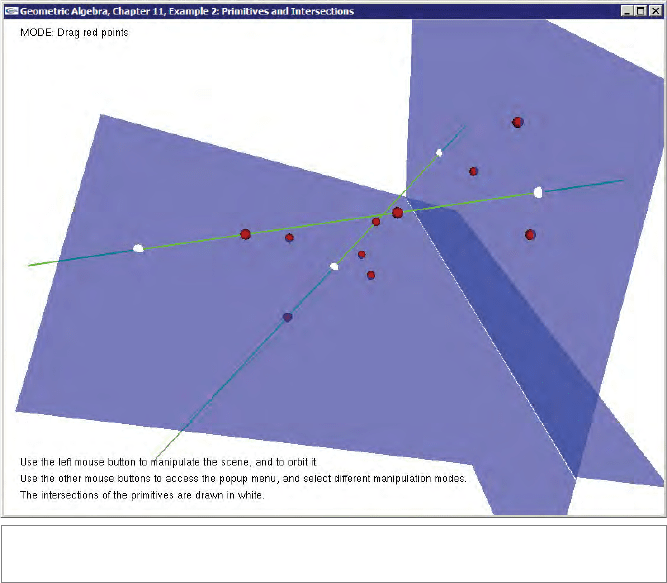
11.13.2 INTERSECTING PRIMITIVES

This example allows you

1. To drag points;

2. To create new points;

3. To combine points to form lines and planes.

The intersections of the lines and planes are computed and dr awn. Figure 11.14 shows a

screenshot.

The points are kept in a global array

g_points. Give two indices (pointIdx1 and

pointIdx2), a line is computed from two points as

line L = _line(g_points[pointIdx1] ^ g_points[pointIdx2]);

The code for computing a plane through three points is very similar:

plane P = _plane(g_points[pointIdx1] ^ g_points[pointIdx2] ^

g_points[pointIdx3]);

The intersections of the lines and planes are computed in a very generic fashion. In prin-

ciple, the code for computing the intersections spells out the

meet:

// compute ’pseudoscalar’ of the space spanned by P1 and P2

mv I = unit_e(join(P1, P2));

// compute P1* . P2

mv intersection = (P1 << inverse(I)) << P2;

Here, P1 and P2 are two primitives (lines or planes). P1 and P2 have been initialized such

that the grade of

P1 is lower than or equal to the grade of P2.

However, this basic code would make it very hard for the user to create degenerate

situations such as two identical lines, a plane and a line contained in it, or a plane con-

tained in a plane. Mouse manipulation will not succeed to bring such situations about.

That is why we use a trick to make the primitives snap to each other. We project

P1 onto

P2. If the projection of P1 is close enough to P1 itself, we set P1 equal to its projection:

mv projection = (P1 << inverse(P2)) << P2;

// check if projection of P1 onto P2 is ’close’ to P1

const float CLOSE = 0.02f;

if (_Float(norm_e(projection — P1)) < CLOSE) {

SECTION11.13 PROGRAMMING EXAMPLES AND EXERCISES 323

// yes:

P1 = projection;

}

Note that this construction will (unfortunately) not snap skew lines to make them

intersect.

Creating Points

The example also allows the user to create points by clicking at any p oint in the viewport.

The user expects a point to be created under the mouse cursor, but the distance from the

viewport is in principle unspeciﬁed; to keep the user interface simple, we assume that

using the distance of the previously dragged point is a good choice.

To implement this, we ﬁrst create a new point at the required

distance from the camera:

// create a new point at ’distance’ from camera

normalizedPoint pt = _normalizedPoint(vectorAtDepth(distance,

mousePos) — e3 * distance);

Figure 11.14: Example 2 in action.

324 THE HOMOGENEOUS MODEL CHAPTER 11

The function vectorAtDepth() returns a the 2-D vector mousePos scaled such that the

projection (at

distance)isequalmousePos. Subtracting e3 * distance then gives the

required point. But this point is still in the camera (modelview) frame.

To transform the point to the global frame, we retrieve the OpenGL modelview matrix,

invert it, and apply it to the point as an outermorphism:

// retrieve modelview matrix from OpenGL:

float modelviewMatrix[16];

glGetFloatv(GL_MODELVIEW_MATRIX, modelviewMatrix);

// invert matrix

float inverseModelviewMatrix[16];

invert4x4Matrix(modelviewMatrix, inverseModelviewMatrix);

// use matrix to initialize an outermorphism; apply it to the point

omPoint M(inverseModelviewMatrix);

pt = apply_om(M, pt);

The point is then added to the global list of points. We will make more use of matrices

and outermorphisms in Sections 12.5.1 and 12.5.2.

11.13.3 DON’T ADD LINES

As described in Section 11.3.3, the sum of two homogeneous lines is another line only

when they have a factor in common. It then is the weighted average of the two lines.

Otherwise, their sum is not a blade, and hence not geometrically interpretable. The fol-

lowing example demonstrates this.

You can drag around the four points that span the lines. The example computes the two

lines and draws them. It also adds the lines, and tries to draw the result:

// compute the lines

line L1 = _line(pt[0] ^ pt[1]);

line L2 = _line(pt[2] ^ pt[3]);

line L1plusL2 = _line(L1 + L2);

// ...

draw(L1);

draw(L2);

// ...

draw(L1plusL2);

L1plusL2

will show up only when

•

L1 and L2 share a point;

•

L1 and L2 have the same direction.

To facilitate creating such situations, the example makes the points snap to each other

SECTION11.13 PROGRAMMING EXAMPLES AND EXERCISES 325

when they get within close range. The example also adjust the directions when the lines

are near-parallel, such that the lines become truly parallel.

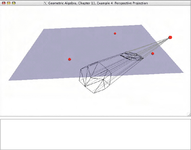
11.13.4 PERSPECTIVE PROJECTION

This example projects 3-D models onto an image plane, as shown in Figure 11.15. The

camera and the image plane are determined by four points:

normalizedPoint cameraPoint = g_points[CAMERA_PT_IDX];

plane imagePlane = _plane(

g_points[IMAGE_PLANE_PT_IDX + 0] ^

g_points[IMAGE_PLANE_PT_IDX + 1] ^

g_points[IMAGE_PLANE_PT_IDX + 2]

);

The points are stored in a global array g_points. They can be dragged around using the

mouse. The projection is perfor med by constructing the line

vertex ∧ cameraPoint

and intersecting it with the imagePlane:

Three red points span the imaging plane, and the fourth represents the camera.

Use the left mouse button to drag the red points, and to orbit the scene.

Use the other mouse buttons access the popup menu (to select a different model, and to toggle rays on/off).

Figure 11.15: Perspective projection (Example 4). The dodecahedron gets projected onto

the blue image plane. This is done by constructing rays (lines) between the vertices of the

dodecahedron and the camera (the red point on the right). The image plane is determined by

the other three points. The meet of rays and plane produces the intersection points.

326 THE HOMOGENEOUS MODEL CHAPTER 11

const normalizedPoint &vertex = g_vertices3D[g_polygons3D[i][j]];

// compute projected vertex

point pv = _point(dual(vertex ^ cameraPoint) << imagePlane);

We perform back-face culling (see also Sec tion 2.13.2), by comparing the orientation of

the image plane with the orientation of the plane spanned by the projected vertices:

// array PV contains the projected vertices

mv::Float ori = _Float((PV[0] ^ PV[1] ^ PV[2]) *

inverse (imagePlane));

if (ori > 0.0f) {

// draw the polygon

// ...

}

Note that when you reverse orientation of the image plane (by reversing the order of the

points that deﬁne it), you get the opposite deﬁnition of which faces are the back-faces.

In that case, you will see the backside of the model projected onto the plane.

(Disclaimer: It is of course faster to use a matri x representation of the projection outer-

morphism, but this example is intended as an enlightening exercise on an alternative geo-

metrical manner to produce the same result.)

Exercise 4a: Orthogonal Projection

Adjust the example to use orthogonal projection rather than perspective projection. Note

that such an orthogonal projection is fully speciﬁed by the image plane, so that the camera

position is irrelevant. The solution to this exercise is not simply to use the orthogonal pro-

jection formula (AB

−1

)B, due to the metric imperfections of the homogeneous model

discussed in Section 11.10.

APPLICATIONS OF THE

HOMOGENEOUS MODEL

The homogeneous model is well suited to applications in which incidences of offset ﬂat

subspaces are central, but less so when metric properties are also important. In this, it

plays a role similar to Grassmann-Cayley algebra. This chapter gives details on its direct

use in applications.

In the ﬁrst part, we discuss the coordinate representations of the homogeneous elements.

This naturally embeds the powerful Pl

ucker coordinates for line computations, which

are seen to be are a natural extension of homogeneous point coordinates (using the outer

product). We show how you can master them and derive new application formulas simply.

Those coordinates for lines, as well as points and planes, permit compact formulation of

the afﬁne transformations as matrices.

In the second part, we give an advanced application of the homogeneous model. It is well

suited to encode the projective geometry involved in the imaging of the world by one

or more pinhole cameras. The homogeneous model permits easy speciﬁcation of how

observations in the various cameras are connected, which permits using observations by

one camera to guide the search for corresponding features in another camera. We treat

the fairly advanced subjects of stereo-vision based on point and line matches in 2 or 3

cameras.

Both subjects of this chapter are incidental to the main ﬂow of the book, though the sec-

tion on Pl

ucker coordinates prepares you for the implementation of geometric algebra in

Part III.

327

328 APPLICATIONS OF THE HOMOGENEOUS MODEL CHAPTER 12

12.1 HOMOGENEOUS PL

UCKER COORDINATES IN 3-D

In the previous chapter, we saw how the homogeneous model permits direct and dual

representation of ﬂats. This extends the commonly used homogeneous coordinates for

points and hyperplanes used throughout computer graphics and robotics literature. In

some more specialized texts, you may also ﬁnd a representation of lines by Pl

ucker coor-

dinates. These are coordinates tailored to the description of lines, and they permit direct

computation w ith lines as basic elements. That provides for faster and simpler code than if

you described lines by a direction vector and a position vector, or as two plane equations,

or by two points. Repeated attempts have been made to introduce them into mainstream

computer graphics, where line computations are obviously impor tant, but with limited

success.

It is clear why Pl

ucker coordinates are less well known than they deser ve to be. In the usual

texts, they are presented as a strange mathematical trick, not clearly related to the homo-

geneous coordinates. They require 6-D vectors and corresponding matrices, which appear

extraneous to the usual 4-D data structures in homogeneous coordinate software. So most

people continue to encode lines as composite elements in a data structure consisting of

two vectors. This denies lines the status of being convenient elements of computation, and

that in turn affects solutions to practical problems; if there is a natural way of describing

and solving some problem using lines, it is less likely to be found. An example is visual

self-localization by a robot in an ofﬁce environment; a ty pical solution looks to match

point features, neglecting the numerous straig ht lines usually present in such an environ-

ment. Reducing every thing to point-based or plane-based computations may be subopti-

mal and neglects the perfectly useful and stably measurable str aight edges. But to actually

use them in your estimation processes, you need the ability to compute with them.

In this chapter, we show how to look at the Pl

ucker coordinates in a manner that makes

them natural and convenient to use. There are no new concepts here; this is an application

of the structure of the previous chapter, but is good to relate the algebra to the speciﬁc

coordinate techniques that the proponents of Pl

ucker coordinates (such as [57]) suggest.

12.1.1 LINE REPRESENTATION

Let us again look at the representation of lines, and focus speciﬁcally on a 3-D base space.

The line representation p ∧ q of (11.3) as

p ∧ q = e

∧ (q − p) + p ∧ q (12.1)

involves six coordinates: three for the 2-blade e

∧ (q − p) and three for the 2-blade p ∧ q.

There is one dependency relationship (since e

∧ (q − p) ∧ (p ∧ q) = 0), and that reduces

the degrees of freedom of the line to ﬁve. Geometrically, you can interpret the ﬁrst term

of (12.1) as the direction vector and the second term as the moment. We have denoted

those in Figure 12.1. This ﬁgure cannot show the fourth dimension e

; with that extra

SECTION 12.1 HOMOGENEOUS PL

UCKER COORDINATES IN 3-D 329

−

p ∧ q

p × q

Figure 12.1: Pl

ucker coordinates of a line in 3-D.

dimension it should look more like Figure 11.2(a), which is its lower-dimensional version

for lines in 2-D.

We can group the six coordinates of a line in 3-D as two vectors of three components, by

employing the cross product:

p ∧ q = e

∧ (q − p) + p ∧ q = (p − q) e

+ (p × q) I

(12.2)

We recognize (minus) the direction vector and the dual of the moment 2-blade (which

is the properly weighted normal vector of the plane through the line and the origin).

Together, these form the Pl

ucker coordinates of the 3-D line, denoted by

−{p − q; p × q}

(12.3)

(see [57]). Classically, these are often treated as six slots for storing numbers, without

much algebraic structure, and manipulations with these numbers may seem rather arbi-

trary, especially when combined with the homogeneous coordinate representations of

points and planes. Table 12.1 gives some examples. The operations are simple and fast

and that explains the interest of the Pl

ucker coordinates, but the structure between these

“magic formulas” is lost, so that implementations are hard to extend to cases not covered

in such tables (or to higher dimensions). The usual nonalgebraic encoding of the type of

element represented by different kinds of brackets around the coordinates does little to

clarify the str ucture of the table.

330 APPLICATIONS OF THE HOMOGENEOUS MODEL CHAPTER 12

Table12.1: Common Pl

ucker coordinate computations with a line {a, m}, a plane [n, δ], and

a point ( p :1). The type of bracket denotes the type of object nonalgebraically. (Expanded from

[57].) Note that a is minus the usual direction vector.

(p :1) Point at location p

[n, − δ] Plane with normal n and offset δ

n · p − δ Distance from point to plane

{a, m} = {p − q, p × q} Line through two points, from Q to P

(m·m )/(a·a) Squared distance of line to origin

(m × a : a · a) Point on line closest to origin

[a × m : m · m] Plane through line, perpendicular to origin plane

(m × n + δ a : a · n) Point in line and plane

[a × p − m : m · p] Plane through line and point

[a × n : m · n] Plane through line, additional direction n

In the geometric algebra point of v iew, we see that the six numbers are coefﬁcients on a

speciﬁc basis, in (12.2) demonstr ated by the extra symbols e

and I

. This gives the full

algebraic meaning to the Pl

ucker coordinates, and endows them automatically with rela-

tionships to the other elements through their membership in geometric algebra. Their

actual construction in (12.2) is a clear instance of this: by taking the outer product of

two homogeneous points, we get the line representation, providing the straightforward

connection between point coordinates and line coordinates through the standard oper-

ation of outer product. The same standard operation should connect the table entries

for point, line, and plane through line and point. This obvious geometrical fact is not

at all clear from the corresponding entries in Table 12.1. Only by translating the bracket

notation back into its actual geometric basis and applying the standard constructions of

geometric algebra can we understand and extend such tables.

12.1.2 THE ELEMENTS IN COORDINATE FORM

In the homogeneous model of 3-D space, the representation of the quantities in terms of

coordinates is easily computed. We give a complete inventory of the repertoire of geomet-

ric elements in the homogeneous model. We study the coordinate representation of the

offset ﬂat subspaces of various grades (points, lines, and planes) in both their direct and

in their dual representations.

1. Point. We have seen that the 1-D homogeneous subspace representing a 0-D point

in the homogeneous model is of the form e

+ p (or a multiple). In a homoge-

neous model of 3-space with basis {e

, e

}, it therefore has the coordinates

SECTION 12.1 HOMOGENEOUS PL

UCKER COORDINATES IN 3-D 331

, p

, 1) (or a multiple), with (p

, p

) the Euclidean coordinates of its

position vector. In Table 12.1 this is w ritten as (p :1), following [57].

2. Hyperplane. If we have a plane characterized as all points x such that x · n = δ,

this can be written as (e

+ x ) · (−n + δe

−1

) = 0,soasx · (−n + δe

−1

) = 0.

Therefore −n + δe

−1

(or any multiple of it) is the dual of the blade representing

the hyperplane. It is represented on a basis {e

, e

−1

}, which appears different

from the basis for points until you realize that e

−1

= ±e

, depending on the metric

chosen. Therefore the bases are the same, and you cannot tell these elements apart

as vectors.

If −n + δe

−1

is the dual of a blade, then the blade itself must be

(−n + δe

−1

)(e

) = −ne

+ δI

(where we take the undualization in the (n + 1)-dimensional homogeneous

model, so relative to the pseudoscalar e

). This has the Pl

ucker coefﬁcients

, n

: −δ] used in Table 12.1, but on the trivector basis

, e

, − e

which is clearly different from the vector basis for points. In standard literature

on Pl

ucker coordinates, this difference in basis is denoted nonalgebraically by

square brackets: [n : −δ]. Others consider planes as row vectors, and points as

column vectors, so then their brackets could be interpreted as specifying this

difference.

If you want a consistent representation of the direct and dual-oriented planes, you

should be very explicit in your choice of basis. The dual plane also has a represen-

tation [n : −δ], but the basis is {−e

, − e

−1

= ∓e

} (the sign of the last

element related to the sign in e

−1

= ±e

). Such headaches are the consequences of

splitting up a single geometr ic element (the dual plane) in its coordinates and basis,

each of which separately have no objective geometric meaning.

3. Lines. We have seen above in (12.2) that a line is represented by minus the usual

direction vector a = p − q andamomentvectorm = p × q = −p × a as

L = a e

+ mI

(12.4)

The six coefﬁcients {a

, a

, m

} of this line are on the bivector basis

, e

(12.5)

In Table 12.1, we follow [57] in using curly br ackets for this data type. In derivations

with lines, we obviously need to revert to the fully expressed form.