Enns R.H. Computer Algebra Recipes for Mathematical Physics

Подождите немного. Документ загружается.

2.3. FOURIER SERIES 77

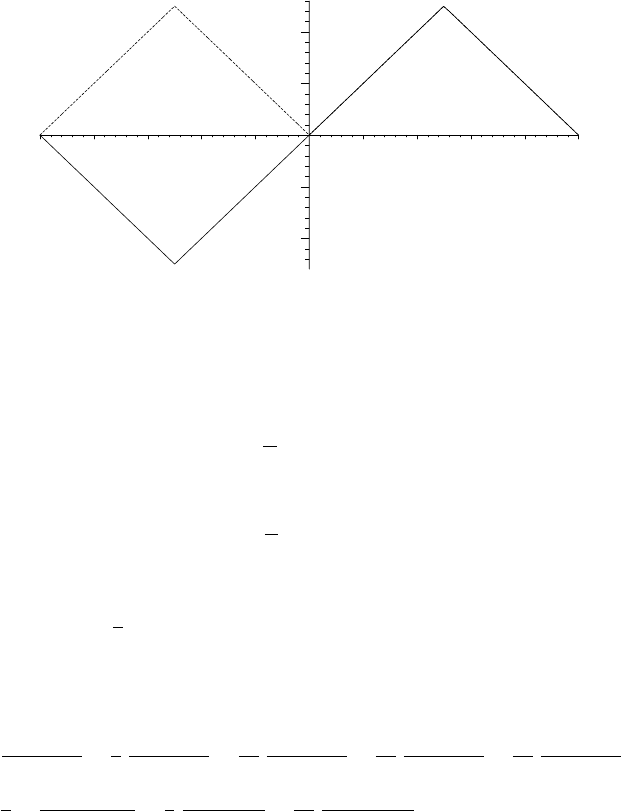
An even function f2 is introduced which is the same as f for 0 ≤ x ≤ L and

symmetrical about the origin. f 2 is used to generate the cosine series.

f2:=piecewise(x<-L/2,L+x,x<0,-x,x<L/2,x,x<L,L-x);

To conﬁrm that f1andf2 are odd and even extensions of f to the region x<0,

they are plotted as solid and dashed curves in Figure 2.6. For x>0, the two

curves are identical, and therefore indistinguishable.

plot([f1,f2],x=-L..L,linestyle=[SOLID,DASH],thickness=2);

–0.4

0.4

–1 1

Figure 2.6: Solid curve, f1. dashed curve, f2.

For a given f , functional operators A, B and F are introduced to calculate the

series coeﬃcients a

and b

, and to produce the series out to N terms.

A:=(f,n)->(1/L)*int(f*cos(n*X),x=-L..L);

A := (f, n) →



−L

f cos(nX) dx

B:=(f,n)->(1/L)*int(f*sin(n*X),x=-L..L);

B := (f, n) →



−L

f sin(nX) dx

F:=(f,N)->A(f,0)/2+sum(A(f,n)*cos(n*X)+B(f,n)*sin(n*X),n=1..N);

F := (f, N) →

A(f, 0) + (



n=1

(A(f, n) cos(nX)+B(f, n)sin(nX)))

Taking N =10, the Fourier sine and cosine series are produced in F1 and F2 .

F1:=F(f1,10); F2:=F(f2,10);

F1:=

4sin(πx)

−

sin(3 πx)

sin(5 πx)

−

sin(7 πx)

sin(9 πx)

F2:=

−

2 cos(2 πx)

−

cos(6 πx)

−

cos(10 πx)

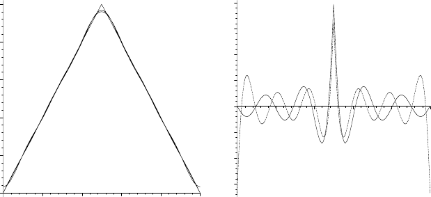
The two series are plotted along with f and shown on the left of Figure 2.7.

plot([f,F1,F2],x=0..L,color=[blue,red,green],thickness=2);

78 CHAPTER 2. APPLICATIONS OF SERIES

0.5

–0.01

0.01

0.02

Figure 2.7: Left: f and the two series. Right: Solid, f −F1. Dashed, f − F2 .

Even though N is not large, both series ﬁt f quite well, except near the apex

of the triangle and, for the cosine series, near x = 0 and 1. To magnify the

diﬀerence between the series results and f, the diﬀerences f − F1 and f − F2

are plotted as solid and dashed curves in the right graph of Figure 2.5.

plot([f-F1,f-F2],x=0..L,linestyle=[1,3],thickness=2);

The cosine series clearly ﬁts less well at the end points of the x range. Can you

suggest why this is the case?

2.3.3 How Sweet This Is!

Few things are harder to put up with than the annoyance

of a good example.

Mark Twain, American author, Pudd’nhead Wilson, 1894

If you have calculated series expansions by hand, you know what a tedious

task it can be to explicitly calculate a large number of terms in the series and

then have to plot the results. By now, you should have gotten a clear idea that

using computer algebra is the way to go in handling such problems. The fol-

lowing recipe for the Legendre–Fourier series is a particularly “sweet” example

that derives a “beautiful” result very quickly.

Consider a step function, f(x)=0for −1 <x<0andf(x) =1 for 0 <x<1.

Derive the Legendre–Fourier series for f and plot the series and f together over

the range −1 <x<1. Calculate the area between the x-axis and the series

curve and compare with the exact result for f. Discuss the plot and area results.

restart:

2.3. FOURIER SERIES 79

Functional operators A and F are formed to calculate the coeﬃcients A

,and

the Legendre series out to N terms, for a given function f.

A:=(f,n)->((2*n+1)/2)*int(f*LegendreP(n,x),x=-1..1);

A := (f, n) →

(2 n +1)



−1

f LegendreP(n, x) dx

F:=(f,N)->sum(A(f,n)*LegendreP(n,x),n=0..N);

F := (f, N) →



n=0

A(f, n) LegendreP(n, x)

The given f is entered with the Heaviside(x) command and the Legendre-

Fourier series calculated in F1 for N =15.

f:=Heaviside(x); F1:=F(f,15);

f := Heaviside(x)

F1 :=

3 x

−

LegendreP(3,x)+

LegendreP(5,x)

−

256

LegendreP(7,x)+

133

512

LegendreP(9,x) −

483

2048

LegendreP(11,x)

891

4096

LegendreP(13,x) −

13299

65536

LegendreP(15,x)

This is a formidable looking series, which has been generated in three command

lines. If I now wanted to see what the series looks like for, say N =100, changing

15 to 100 in F1 and executing the command would generate the new result

almost instantaneously.

How formidable the result really is, even for 15 terms, can be appreciated by

expanding F1 .Thesort command is used to order the polynomial expansion

from the highest exponent to the lowest. Wow, what a result!

F1:=sort(expand(F1));

F1 := −

128931743655

134217728

503889568875

134217728

−

800852700375

134217728

664630841875

134217728

−

307629132525

134217728

78646056489

134217728

−

10402917525

134217728

703956825

134217728

x +

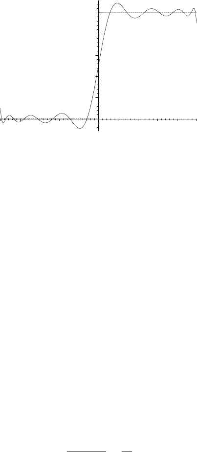
Now f and F1 are plotted in Figure 2.8 over the range x = −1to1,andare

represented by dashed and solid curves, respectively.

plot([f,F1],x=-1..1,thickness=2,linestyle=[3,1]);

Two features of the Legendre series are quite clear from the picture, and can be

conﬁrmed by taking N larger. (You will have to adjust the view and number

of digits and plotting points.) The series curve displays a Gibb’s phenomenon

and also passes through the midpoint of the step.

80 CHAPTER 2. APPLICATIONS OF SERIES

–1 1

Figure 2.8: Dashed curve, Step function f. Solid curve, Legendre series F1 .

The area between the Legendre series curve and the x-axis is now calculated

and found to be exactly the same as the area for the step function.

Area:=int(F1,x=-1..1);

Area := 1

2.4 Summing Series

In this section, two diﬀerent approaches to summing inﬁnite series are presented.

The ﬁrst recipe makes use of ideas already introduced in the earlier Fourier

series examples. In the second recipe, the series to be summed is replaced by a

complexserieswhichMapleisabletosum.

2.4.1 I. M. Curious Sums a Series

Once, I thought I made a mistake, but I was mistaken.

From the diary of I. M. Curious

In this recipe, Ms. Curious answers the following question:

By expanding f(x)=x(L − x), deﬁned in the interval (0,L)withL= π,in

a Fourier sine series of period 2L and setting x = L/2, prove that

∞



n=0

(−1)

(2n +1)

Conﬁrm this result by directly summing the series with Maple, ﬁrst showing

that the sum can be expressed as either a generalized hypergeometric function

or as a polylogarithm function.

I. M. begins her solution by assuming that the Fourier series summation

indices m and n are integers. She then sets L=π and enters f =x (L − x).

2.4. SUMMING SERIES 81

restart: assume(m::integer,n::integer):

L:=Pi: f:=x*(L-x):

To expand f in a Fourier sine series of period 2 L, she forms the following odd

piecewise function, pw, deﬁned in the interval −L<x<L.

pw:=piecewise(x<0,x*(L+x),x>0,f);

pw :=



x (π + x) x<0

x (π − x)0<x

I. M. then calculates the Fourier coeﬃcients a

, a

for m =0,andb

a[0]:=(1/L)*int(pw,x=-L..L);

:= 0

a[m]:=(1/L)*int(pw*cos(m*Pi*x/L),x=-L..L);

:= 0

b[m]:=(1/L)*int(pw*sin(m*Pi*x/L),x=-L..L);

:= −

4(−1+(−1)

)

πm

She notices that in b

the coeﬃcients are only non-zero if m is an odd integer.

So she substitutes m =2n +1 into b

and relabels the coeﬃcients as b

2n+1

The new summation index n will take on the values n =0, 1, 2, ....

b[2*n+1]:=simplify(subs(m=2*n+1,b[m]));

2 n+1

π (2 n +1)

Since the coeﬃcients a

are zero for all m (and therefore all n), the Fourier

series is then of the form F =



∞

n=0

2n+1

sin((2n +1)πx/L).

F:=Sum(b[2*n+1]*sin((2*n+1)*Pi*x/L),n=0..infinity);

F :=

∞



n=0

(

8 sin((2 n +1)x)

π (2 n +1)

)

Thus, the original function f in the region 0 <x<Lcanbewrittenasthe

Fourier sine series F .Thisisenteredineq1 .

eq1:=f=F;

eq1 := x (π − x)=

∞



n=0

(

8 sin((2 n +1)x)

π (2 n +1)

)

eq1 is divided by 8 and evaluated at x=L/2.

eq2:=eval(eq1/8,x=L/2);

eq2 :=



∞



n=0

(

8(−1)

π (2 n +1)

)



Multiplying eq2 by π, and expanding, conﬁrms the series sum.

eq3:=expand(Pi*eq2);

82 CHAPTER 2. APPLICATIONS OF SERIES

eq3 :=

∞



n=0

(−1)

(2 n +1)

To sum the series directly with Maple, I. M. extracts it from the rhs of eq3 .

S:=rhs(eq3);

S :=

∞



n=0

(−1)

(2 n +1)

She expresses the sum S as a hypergeometric function by applying the following

convert command.

S:=convert(S,hypergeom);

S := hypergeom([

, 1], [

], −1)

If this function is unfamiliar to you, highlight hypergeom in the computer out-

put with your mouse and open the relevant help window to see its deﬁnition.

According to Help, it may be possible to convert the hypergeometric function

into one of the standard special and elementary functions found in such texts

as Handbook of Mathematical Functions by Abramowitz and Stegun ([AS72]).

Applying the convert(StandardFunctions) command,

S:=convert(S,StandardFunctions);

S := −

I polylog(3,I)+

I polylog(3, −I)

yields a combination of polylog functions. Again, if the polylogarithm function

is unfamiliar, it may be looked up in Maple’s Help. I. M. ﬁnally obtains the

desired form of the series sum by using simplify.

S:=simplify(S);

S :=

2.4.2 Spiegel’s Series Problem

Old age is that time of life when you can feel bad in the morning

without having had fun the night before.

Gregarius Nerd, Professor of Mathematics, Erehwon Institute of Technology

In the previous example, we saw that Maple was successful in summing the

given series. If Maple is unsuccessful, does that mean that the series cannot be

summed? Not necessarily, as you will now see. Sometimes it needs a bit of help

in the form of human brain power. This will not be the last time in this book

that this is the case.

Let’s consider the following inﬁnite series,

r sin(φ)+

sin(3 φ)+

sin(5 φ)+

sin(7 φ)+···, (2.13)

which, according to the Schaum Outline Series on Advanced Mathematics by

Murray Spiegel ([Spi71]), arises from solving for the steady-state temperature

2.4. SUMMING SERIES 83

distribution in a thin circular plate of unit radius whose faces are insulated and

has each half of its boundary kept at a diﬀerent constant temperature. In polar

coordinates, r is the radial distance from the center of the plate and φ the polar

angle. Spiegel’s Problem 12.52 is to show that the series can be summed and

cast into the form (1/2) tan

−1

(2r sin φ/(1 − r

)).

The following recipe solves Spiegel’s problem. An operator S is formed to

generate the series out to exponent 2 N +1.

restart:

S:=N->sum(rˆ(2*m+1)*sin((2*m+1)*phi)/(2*m+1),m=0..N);

S := N →



m=0

(2 m+1)

sin((2 m +1)φ)

2 m +1

Taking N =3, then entering S(3) generates the terms displayed in (2.13).

S1:=S(3);

S1 := r sin(φ)+

sin(3 φ)+

sin(5 φ)+

sin(7 φ)

Taking N = ∞ in S and applying the value command, we ﬁnd that Maple is

unable to directly sum the series, returning the unevaluated sum in S2 .

S2:=value(S(infinity));

S2 :=

∞



m=0

(2 m+1)

sin((2 m +1)φ)

2 m +1

To sum the series, note that the real series can be written as the imaginary part

of a complex series. To accomplish this, the summand in S2 can be taken as

the imaginary part of a complex summand, viz., with I ≡

√

−1,



2m+1

I(2m+1)φ

2m +1



=Im



(re

Iφ

)

2m+1

2m +1



=Im



2m+1

2m +1



with z ≡re

Iφ

. Using this result, the complex series, CS, is entered and then

successfully summed.

CS:=Sum(zˆ(2*m+1)/(2*m+1),m=0..infinity);

CS :=

∞



m=0

(2 m+1)

2 m +1

CS:=value(CS);

CS :=

ln(

1+z

1 − z

)

Then, z =re

Iφ

is substituted into CS,

CS2:=subs(z=r*exp(I*phi),CS);

CS2 :=

ln(

1+re

(φI)

1 − re

(φI)

)

and the complex result CS2 broken into real and imaginary parts in CS3 with

the complex evaluation command and simpliﬁed in CS4 assuming r<1.

84 CHAPTER 2. APPLICATIONS OF SERIES

CS3:=evalc(CS2);

CS4:=simplify(CS3) assuming r<1;

CS4 :=

ln(

+2r cos(φ)+1

1 − 2 r cos(φ)+r

)

I arctan(

2 r sin(φ)

1 − 2 r cos(φ)+r

, −

−1+r

1 − 2 r cos(φ)+r

)

The portion of the argument in arctan before the comma is the numerator, the

portion after the comma being the denominator. To extract the imaginary part

of CS4 ,thecoeff command is used to pull out the coeﬃcient of I.

S3:=coeff(CS4,I);

S3 :=

arctan(

2 r sin(φ)

1 − 2 r cos(φ)+r

, −

−1+r

1 − 2 r cos(φ)+r

)

The operand command, op is used to write the series sum in a form which

agrees with the result quoted by Spiegel.

S4:=op(1,S3)*arctan((op([2,1],S3)/op([2,2],S3)));

S4 := −

arctan(

2 r sin(φ)

−1+r

)

2.5 Supplementary Recipes

02-S01: Euler and Bernoulli Numbers

(a) Taylor expand sec(z), dropping terms of O(z

). The Euler numbers E

are deﬁned by sec(z)=



∞

n=0

(−1)

/(2n)! Using the Euler number

command euler(2*n), conﬁrm that the latter expansion of sec(z) agrees

with the Taylor expansion. Generate the Euler numbers E

,...,E

(b) Taylor expand z/(e

−1), dropping terms of O(z

). The Bernoulli num-

bers B

are deﬁned by z/(e

− 1) =



∞

n=0

/n! Using the Bernoulli

number command bernoulli(n), conﬁrm that the latter expansion agrees

with the Taylor expansion. Generate the ﬁrst 10 Bernoulli numbers.

02-S02: Ms. Curious Approximates an Integral

Ms. Curious has been given the following problem to solve. Consider the integral

f(x)=



sin(t

) dt. Evaluate this integral analytically and identify the function

which occurs. Obtain the smallest polynomial approximation to f(x)whichis

valid within ±0.00001 for 0 ≤ x ≤ 1.

02-S03: More Finite Diﬀerence Approximations

(a) Conﬁrm the following ﬁnite diﬀerence approximation,



(x)=[y(x +2h) −4y(x + h)+6y(x) − 4y(x − h)+y(x − 2h)]/h

Suggest a physical problem for which this FDA might be useful. Taking

y = x

4.7

, graphically compare and discuss the FDA (with h =0.1and12

digits accuracy) with the exact 4th derivative over the range x=0 to 70.

2.5 SUPPLEMENTARY RECIPES 85

(b) Show that an FDA to the Laplacian, ∇

f(x, y)≡∂

f/∂x

+∂

f/∂y

,is

∇

f(x, y)=(1/12 h

)[16 [f(x+h, y)+f (x, y+h)+f(x − h, y)+f (x, y − h)]

−[f(x+2h, y)+f (x, y+2 h)+f(x − 2 h, y)+f (x, y −2 h)+60f(x, y)]].

Suggest a physical problem for which this FDA might be useful. Consid-

ering f(x, y)=e

−x

and taking h =0.1 and 10 digits accuracy, produce

a 3-dimensional color-coded plot of the diﬀerence between the exact 2-

dimensional Laplacian and the FDA for the range x = −2..2, y = −2..2.

02-S04: Series Solution

Mimicking a hand calculation, obtain a general series solution, valid near x=0,

of the following LODE



+2y



+ xy =0.

Show that the series solution may be expressed in a closed form. Conﬁrm this

closed-form solution by directly solving the LODE with the dsolve command.

02-S05: Chebyshev Polynomials Revisited

Obtain a general series solution of Chebyshev’s equation,

(1 − x

) y



− xy



+ p

y =0

valid near x = 0, by (a) mimicking a hand calculation, (b) using the series

option in the dsolve command. If p is a positive integer, show that one or

the other of the series in the general solution reduces to a ﬁnite polynomial.

These polynomials are the Chebyshev polynomials. The zeroth order Chebyshev

polynomial T

(x) = 1. The higher order polynomials T

(x) are normalized so

that the coeﬃcient of the largest power in the mth order polynomial is 2

(m−1)

Derive the Chebyshev polynomials T

, T

, ..., T

and plot T

to T

over the

range x = −1 to 1. Note that the non-ﬁnite-polynomial parts of the solution

diverge at the end points of the range and are rejected in physical problems.

02-S06: A Fourier Series

Expand f(θ)=θ

,0<θ<2 π, in a Fourier series F of period 2 π.Plotf and

F (for an upper value N =20 of the summation index) in the same ﬁgure.

02-S07: Fourier Sine Series

Taking L =1,expandeachofthefollowingf(x) in a Fourier sine series F of

period 2L, over the interval (0, L):

(a) f (x)=x (L − x);

(b) f (x)=x,0<x<L/2, and f (x)=L − x, L/2<x<L;

In each case plot f(x)andF (for an upper value N = 10 of the summation

index) in the same ﬁgure and discuss the goodness of the ﬁt.

02-S08: Fourier Cosine Series

Taking L=1,expandeachofthef(x) given in 02-S07 in a Fourier cosine series

86 CHAPTER 2. APPLICATIONS OF SERIES

F of period 2L, over the interval (0, L). In each case plot f(x)andF (for an

upper value N =10 of the summation index) in the same ﬁgure and discuss the

goodness of the ﬁt.

02-S09: Legendre Series

Expand the following f(x) in a series F of Legendre polynomials (up to n =

N =15) and plot f and F together in the same ﬁgure:

(a) f (x)=0, −1<x<0, and f(x)= 1, 0<x<1;

(b) f (x)=0, −1<x<0, and f(x)=x,0<x<1.

02-S10: Directly Evaluating Series Sum

Write the following inﬁnite series out in the summation notation and then use

Maple to directly evaluate the series sum in closed form:

(a) f (x)=1+2x +3x

+4x

+ ···

(b) f (x)=

1 · 2

2 · 3

3 · 4

4 · 5

+ ···

1 · 3

2 · 4

3 · 5

4 · 6

+ ···

(d) f (x)=x −

4 x

9 x

−

16 x

+ ···

02-S11: Another Cosine Series

Expand f(x)=sin(x), 0 <x<π, in a Fourier cosine series F . Explicitly write

out F for the ﬁrst 5 non-zero terms and plot F and f(x) together. Use F to

prove



∞

n=1

1/(4n

−1)= 1/2. Conﬁrm this by directly summing with Maple.

02-S12: The Complex Series Trick Again

In a certain 2-dimensional electrostatic potential problem, the following inﬁnite

series occurs:

S =sin(

πx

) e

−

πy

sin(

3 πx

) e

−

3 πy

sin(

5 πx

) e

−

5 πy

+ ···

Show that the series can be summed and put into the form

S =

arctan



sin(πx/a)

sinh(πy/a)

