Enns R.H. Computer Algebra Recipes for Mathematical Physics
Подождите немного. Документ загружается.


Chapter 3
Vectors and Matrices
In the first section of this chapter, we see how Maple may be used to deal with
vectors in Cartesian coordinates. Examples of vector algebra, the dot and cross
products, the gradient operator, and vector identities are presented.
The second section extends the discussion to vectors in orthogonal
1
curvi-
linear coordinate systems such as spherical polar, cylindrical, and others. The
vector operators gradient, divergence, curl, and Laplacian are considered and
various important identities and theorems are illustrated.
The third section looks at the manipulation of matrices. Examples of matrix
addition and multiplication, calculating the transpose and inverse and eigen-
values and eigenvectors, and diagonalizing and rotating matrices, are provided.
3.1 Vectors: Cartesian Coordinates
For Cartesian coordinates x, y,andz, the unit vectors ˆe
x
,ˆe
y
,andˆe
z
always
point along the x, y,andz axes for every point in space. A general vector
A
is of the form
A = A
x
ˆe
x
+ A
y
ˆe
y
+ A
z
ˆe
z
.If
A is a function of the coordinates,
then
A is called a vector field.
The sum of two vectors
A and
B is given by
A +
B =(A
x
+ B
x
)ˆe
x
+(A
y
+ B
y
)ˆe
y
+(A
z
+ B
z
)ˆe
z
.
The dot or scalar product between two vectors
A and
B is defined by
A ·
B =AB cos θ,
where A =
A
2
x
+ A
2
y
+ A
2
z
and B =
B
2
x
+ B
2
y
+ B
2
z
are the magnitudes of
A
and
B, respectively.
The cross or vector product of
A and
B, written as
A ×
B, is another vector
whose magnitude |
A ×
B| = AB sin θ. The direction of
A ×
B is given by
the right-hand rule. Put the fingers of the right hand along
A and curl them
towards
B in the direction of the smaller angle between
A and
B. The thumb
then points in the direction of the new vector.
1
The angle between the unit vectors is 90
◦
.

88 CHAPTER 3. VECTORS AND MATRICES
3.1.1 Bobby Blowfly
When you wanted to go Somewhere, And ended up going Nowhere,
The chances are strong, That you were heading for Erehwon.
An anonymous bard
So that he can better survey the goodies on the various picnic tables below
him, Bobby Blowfly is spiraling upwards along a trajectory described by the
Cartesian coordinates x=2 cos(t), y =sin(t), and z =2t/3, where z (in meters)
is measured upwards and t is the time in seconds.
(a) Forming Bobby’s position vector r, calculate his velocity v, acceleration
a, and speed V at time t.
(b) Determine r, v, a,andV at t =3.1and17.3s.
(c) Calculate the magnitude of his displacement for the interval 3.1 to 17.3 s.
(d) Calculate the distance he travels along the spiral path during the interval.
(e) Calculate the angle in radians and degrees between the velocity vectors
at the two times.
(f) Produce a 3-dimensional plot of his trajectory over the time interval with
his velocity and acceleration vectors indicated by arrows at the two times.
To solve this vector problem, the VectorCalculus library package is loaded.
When combined with the plots package, several warning messages will appear
on execution of the following command line which, recall, can be removed by
preceding the package commands with interface(warnlevel=0).
>
restart: with(plots): with(VectorCalculus):
Bobby’s x, y,andz coordinates at time t are entered.
>
x:=2*cos(t): y:=sin(t): z:=2*t/3:
Bobby’s position vector r is entered, using the short-hand
2
syntax <x,y,z>,
and his velocity v and acceleration a are calculated. Note that vector symbols
are not used in the Maple entries.
>
r:=<x,y,z>; v:=diff(r,t); a:=diff(r,t,t);
r := 2 cos(t)e
x
+sin(t)e
y
+
2 t
3
e
z
v := −2sin(t)e
x
+ cos(t)e
y
+
2
3
e
z
a := −2 cos(t)e
x
− sin(t)e
y
Since no coordinate system has been specified, the default output is expressed in
terms of the Cartesian unit vectors e
x
,e
y
,ande
z
. On the computer screen, these
symbols are bold-faced. Using the DotProduct command in the VectorCalculus
package, Bobby’s speed V =
√
v ·v is calculated. The “long form” of this
command is used here. A short-hand syntax will be introduced shortly.
>
V:=sqrt(DotProduct(v,v));
2
A longer form is Vector([x,y,z]).

3.1. VECTORS: CARTESIAN COORDINATES 89
V :=
1
3
4+36sin(t)
2
+ 9 cos(t)
2
The two times, T1 =3.1 s and T2 =17.3 s, are specified and an arrow operator
F formed for evaluating an arbitrary specified function f at a time t =T .
>
T1:=3.1: T2:=17.3: F:=(f,T)->eval(f,t=T):
Making use of F,thenr, v, a,andV are determined at time T1 ,
>
r1:=F(r,T1); v1:=F(v,T1); a1:=F(a,T1); V1:=F(V,T1);
r1 := (−1.998270301) e
x
+0.04158066243 e
y
+2.066666667 e
z
v1 := (−0.08316132486) e
x
− 0.9991351503 e
y
+
2
3
e
z
a1 := 1.998270301 e
x
− 0.04158066243 e
y
V1 := 1.204006353
and at time T2 (output suppressed here).
>
r2:=F(r,T2); v2:=F(v,T2); a2:=F(a,T2); V2:=F(V,T2);
Bobby’s displacement
R = r2 − r1 in the time interval T2 − T1 is calculated
(output suppressed) along with its magnitude Rmag =
R ·
R. To mimic the
hand notation, the short-hand dot syntax is now used to enter the dot product.
Inserting spaces before and after the dot help to distinguish the dot product
from a decimal point and make for easier readability.
>
R:=r2-r1: Rmag:=sqrt(R . R);
Rmag := 9.739961509
The magnitude of Bobby’s displacement in the time interval is about 9.7 meters.
The distance d that he travels along the path is obtained by calculating the
integral
T2
T1
Vdt,
>
d:=int(V,t=T1..T2);
d := 23.93269942
and is found to be about 24 meters. This distance is considerably more than
the magnitude of the displacement.
From the definition of the dot product, the angle θ between the velocities v1
and v2 at times T1 and T2 is obtained by calculating arccos((v1 ·v2 )/(V1 V2 )),
where V1 and V2 are the speeds.
>
theta:=arccos((v1 . v2)/(V1*V2));
θ := 1.469381108
The angle between v1 and v2 is about 1.47 radians or, on converting from
radians to degrees, about 84
◦
.
>
theta2:=convert(theta,units,radian,degree);
θ2 := 84.18933595
A 3-dimensional plot of Bobby’s trajectory over the time interval T1 to T2
is produced with the spacecurve command. To obtain a smooth curve, 500
plotting points are used. The shading=Z option is used to vary the color of the
trajectory with increasing vertical height z.
>
gr||1:=spacecurve([x,y,z],t=T1..T2,numpoints=500,shading=Z):
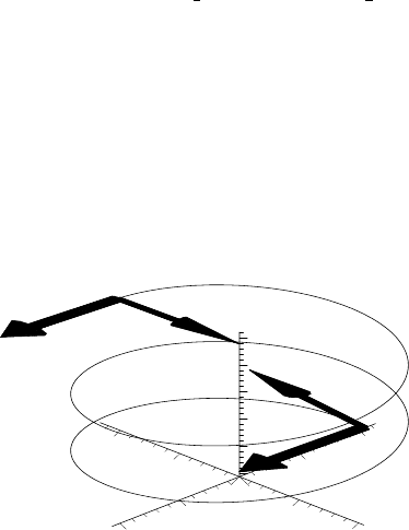
90 CHAPTER 3. VECTORS AND MATRICES
A functional operator f is formed, involving the arrow command, to produce a
cylindrically shaped arrow representing the vector B with its tail at A.Thecolor
c of the arrow must also be provided. The width of the arrow’s “body” as well
as its head width and head length are specified. These values are obtained by
trial and error on viewing the final figure.
>
f:=(A,B,c)->arrow(A,B,shape=cylindrical_arrow,color=c,
width=0.1,head
width=0.3,head length=0.5):
Then f is used to produce a green arrow for the velocity v1 with its tail at r1 ,
a green arrow for v2 with its tail at r2 , a red arrow for the acceleration a1
with its tail at r1 , and a red arrow for a2 with its tail at r2 .
>
gr||2:=f(r1,v1,green): gr||3:=f(r2,v2,green):
gr||4:=f(r1,a1,red): gr||5:=f(r2,a2,red):
Using the sequence command, seq, the five graphs are put into a Maple set and
superimposed in Figure 3.1 with the display command.
>
display({seq(gr||i,i=1..5)},axes=normal,labels=["x","y","z"]);
z
12
–1
1
y
–2
2
x
Figure 3.1: Bobby’s spiral path with v and a at T1 and T2 shown.
As expected, the velocity vectors are tangent to the trajectory, while the ac-
celeration vectors point to the center of the helix. The 3-dimensional plot may
be rotated on the computer screen by dragging with the mouse. It should be
noted that the plot has not been constrained.
3.1.2 Hiking in the Southern Chilkotin
How can you tell that “plop” on the trail is due to a grizzly bear?
It’s full of hiker’s “bear bells” and pepper spray.
Variation on an anonymous backpacker’s saying, R.I.P.
Over the years, I have been fortunate to hike and backpack throughout western
North America, in the mountains of Peru and southern Australia, and in the
jungles of Indonesia. Despite my encounters with a timber wolf, a giant grizzly
3.1. VECTORS: CARTESIAN COORDINATES 91
bear and many not-so-cuddly black bears, one of my favorite backpacking areas
is in the southern Chilkotin area of southwestern British Columbia. This region
marks the transition zone from the wet coastal rain forest with jagged glaciated
peaks to the west and the drier aspen covered slopes climbing towards smoother
reddish brown volcanic tops to the east. This recipe is inspired by my treks in
the southern Chilkotin.
After loading the plots and VectorCalculus packages, the height profile h of
a representative trekking region is entered. Positive x is to the east, positive y
to the north, with all distances in km.
>
restart: with(plots): with(VectorCalculus):
>
h:=(xˆ2+yˆ2)*exp(-0.5*(xˆ2+yˆ2))+1.2*exp(-(x-2.9)ˆ2-(y-2)ˆ2);
h := (x
2
+ y
2
) e
(−0.5 x
2
−0.5 y
2
)
+1.2 e
(−(x−2.9)
2
−(y−2)
2
)
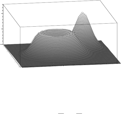
To visualize the terrain, a 3-dimensional contour plot of h is produced over the
horizontal range x = −4to5andy = −4to5,with30contoursshown. The
default is 8 contours. If desired, the heights of the contours can be specified.
The option filled=true fills in the surface of the terrain. The color shading is
varied in the z direction. A particular angular orientation has been chosen for
the plot, but the computer picture may be rotated by dragging with the mouse.
The scaling has been left unconstrained to emphasize the vertical features.
>
contourplot3d(h,x=-4..5,y=-4..5,contours=30,filled=true,
shading=z,axes=box,view=[-4..5,-4..5,0..1.3],
tickmarks=[2,3,3],orientation=[-100,60]);
Figure 3.2 shows a volcanic crater with an adjacent hill. Although the location
0
5
x
–4
0
4
y
0
1
Figure 3.2: Contour plot of trekking region.
and height of the top of the hill can be approximately determined from the
picture, more precise values may be found by using the gradient operator, viz.,
grad h ≡∇h =
∂h
∂x
ˆe
x
+
∂h
∂y
ˆe
y
.

92 CHAPTER 3. VECTORS AND MATRICES
At the top of the hill, the gradient is zero. The Gradient command is used to
calculate grad h at an arbitrary point (x, y). Alternately, one can obtain the
same result by using Del to calculate ∇h.
>
G:=Gradient(h,[x,y]); #alternately, G:=Del(h,[x,y]);
G := (2 xe
(−0.5 x
2
−0.5 y
2
)
− 1.0(x
2
+ y
2
) xe
(−0.5 x
2
−0.5 y
2
)
+1.2(−2 x +5.8) e
(−(x−2.9)
2
−(y−2)
2
)
) e
x
+(2ye
(−0.5 x
2
−0.5 y
2
)
− 1.0(x
2
+ y
2
) ye
(−0.5 x
2
−0.5 y
2
)
+1.2(−2 y +4)e
(−(x−2.9)
2
−(y−2)
2
)
) e
y
Notice that overbars appear above the unit (basis) vectors in the output of
the gradient operation. This indicates that G is a vector field defined at all
points (x, y). It is Maple’s way of reminding you that for general curvilinear
coordinate systems, such as the spherical polar system, the directions of the
unit vectors will vary from point to point in space. Only Cartesian unit vectors
are independent of position.
Guided by the figure, a numerical search is made over the range x = 2 to 4
and y = 1 to 4, using the floating point solve command, to find the zeros of the
x and y components (G[1] and G[2])ofG. The solution sol is assigned,
>
sol:=fsolve({G[1],G[2]},{x,y},{x=2..4,y=1..4}); assign(sol):
sol := {y =1.980898405,x=2.872302687}
and the x and y coordinates of the peak of the hill are given by xmax and ymax.
The height of the hill, hmax, is obtained by evaluating h at xmax, ymax .
>
xmax:=x; ymax:=y; hmax:=eval(h,{x=xmax,y=ymax});
xmax := 2.872302687 ymax := 1.980898405 hmax := 1.226303365
The elevation of the hill’s peak is about 1226 m. x and y are now unassigned.
>
unassign(’x’,’y’):
Topographical maps used in hiking are 2-dimensional in nature. A 2-d contour
map with 25 contours is now made in cp with contourplot.Thegrid option is
set to 50 × 50, which generates 2500 equally spaced grid points for the contour
plot. The default is 25 × 25, which produces 625 grid points.
>
cp:=contourplot(h,x=-4..5,y=-4..5,contours=25,grid=[50,50],
filled=true):
The fieldplot command is used in fp to plot the gradient G, placing thick
magenta colored arrows at equally spaced grid points (here 15 × 15), each arrow
pointing in the direction of increasing gradient at the grid point. The size of the
arrow is a measure of the strength of the gradient, larger arrows corresponding
to steeper gradients.
>
fp:=fieldplot(G,x=-4..5,y=-4..5,arrows=THICK,grid=[15,15],
color=magenta):
The textplot command is used in tp to place the word “Top”, colored blue,
at the location xmax −0.3, ymax +0.1, adjacent to the top of the hill.
>
tp:=textplot([[xmax-0.3,ymax+0.1,"Top"]],color=blue):
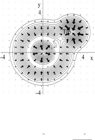
3.1. VECTORS: CARTESIAN COORDINATES 93
After stopping for lunch at the location (xmax −2, ymax − 1.6) near the lip of
the crater, it is desired to hike to the top of the hill. The pointplot command
is used in pp to place size 16 green circles on the contour map at these locations.
>
pp:=pointplot([[xmax,ymax],[xmax-2,ymax-1.6]],
symbol=circle,symbolsize=16,color=green):
The four graphs, fp, cp, tp,andpp, are superimposed with the display com-
mand, the resulting plot being shown in Figure 3.3.
>
display([fp,cp,tp,pp],tickmarks=[3,5]);
Figure 3.3: Two-dimensional contour plot with gradient arrows.
As exp ected, the gradient arrows are perpendicular to the contour lines. The
gradient at the starting point xmax − 2, ymax − 1.6 is determined.
>
G2:=eval(G,{x=xmax-2,y=ymax-1.6});
G2 := 0.6124645476
e
x
+0.2695348694 e
y
The slope at this point is obtained by calculating
G2 ·
G2.
>
Slope:=sqrt(G2 . G2);
Slope := 0.6691501086
The slope is about 0.67. It is positive, in agreement with the figure, indicating
that if we follow the gradient we will b e initially climbing upwards from just
inside the lip of the crater. The slope can be expressed in radians by taking the
arctangent of the slope, which then can be converted to degrees.
>
angle:=arctan(Slope);
angle := 0.5897199394
>
angle:=convert(angle,units,radian,degree);
angle := 33.78846362
94 CHAPTER 3. VECTORS AND MATRICES
Initially we would be climbing at an angle of about 0.6 radians or 34
◦
with
the horizontal. The initial direction of travel can be qualitatively deduced from
Figure 3.3. Quantitatively, the angle in radians measured with respect to the
x-axis (east) can be determined by calculating the arctangent of the ratio of
the y component of G2 to the x component.
>
angle2:=evalf(arctan(G2[2]/G2[1]));
angle2 := 0.4145759092
The angle is about 0.41 radians or, on converting to degrees,
>
angle2:=convert(angle2,units,radian,degree);
angle2 := 23.75344988
about 24 degrees with respect to the easterly direction.
3.1.3 Establishing These Identities is Easy
Trying to define yourself is like trying to bite your own teeth.
Alan Watts, American philosopher on identity, (1915–73)
Vector identities play an important role in many areas of mathematical physics,
particularly in electromagnetism. This recipe illustrates some examples involv-
ing dot and cross products in Cartesian coordinates.
Prove the following identities in Cartesian coordinates for arbitrary
A,
B,
C:
(a)
A · (
B ×
C)=(
A ×
B) ·
C
(b)
A × (
B ×
C)=
B(
A ·
C) −
C(
A ·
B)
(c) [
A × (
B ×
C)]+[
B × (
C ×
A)]+[
C × (
A ×
B)]=0
(d) (
B ×
C) × (
C ×
A)=
C(
A · (
B ×
C))
The VectorCalculus package is loaded and arbitrary vectors
A,
B,
C entered.
>
restart: with(VectorCalculus):
>
A:=<Ax,Ay,Az>; B:=<Bx,By,Bz>; C:=<Cx,Cy,Cz>;
A := Ax e
x
+ Ay e
y
+ Az e
z
B := Bx e
x
+ By e
y
+ Bz e
z
C := Cx e
x
+ Cy e
y
+ Cz e
z
Using the long forms of the dot and cross product commands, the difference
between the left-hand and right-hand sides in (a) is calculated in id1 .
>
id1:=DotProduct(A,CrossProduct(B,C))
-DotProduct(CrossProduct(A,B),C);
id1 := Ax (By Cz −Bz Cy)+Ay (Bz Cx −Bx Cz)+Az (Bx Cy − By Cx)
− (Ay Bz −Az By) Cx − (Az Bx − Ax Bz ) Cy − (Ax By −Ay Bx ) Cz
Applying simplify to id1 yields zero, thus confirming the first identity.
>
id1:=simplify(id1);

3.1. VECTORS: CARTESIAN COORDINATES 95
id1 := 0
For the remainder of the identities, the short-hand syntax for the dot and
crossproducts will be used. We have already used the dot notation for the dot
product. The short form for the cross product is &x. To prove the second
identity
3
in (b), the left-hand side of the identity is now entered. Again, for
clarity, I have left spaces around the cross product symbols.
>
LHS:= A &x (B &x C);
LHS := (Ay (Bx Cy − By Cx) − Az (Bz Cx − Bx Cz )) e
x
+(Az (By Cz −Bz Cy) −Ax (Bx Cy −By Cx )) e
y
+(Ax (Bz Cx −Bx Cz) − Ay (By Cz − Bz Cy)) e
z
Similarly, the right-hand side is entered.
>
RHS:=B*(A . C) - C*(A . B);
RHS := ((Ax Cx + Ay Cy + Az Cz ) Bx − (Ax Bx + Ay By + Az Bz ) Cx)e
x
+((Ax Cx + Ay Cy + Az Cz ) By − (Ax Bx + Ay By + Az Bz ) Cy)e
y
+((Ax Cx + Ay Cy + Az Cz ) Bz − (Ax Bx + Ay By + Az Bz ) Cz )e
z
On simplifying LHS −RHS, a zero vector results in id2, thus confirming (b).
>
id2:=simplify(LHS - RHS);
id2 := 0 e
x
The remaining two identities in (c) and (d) areproveninasimilarmanneras
shown in id3 and id4 , respectively. For the latter, the difference between the
left-hand and right-hand sides is calculated.
>
id3:=(A &x (B &x C)) + (B &x (C &x A)) + (C &x (A &x B));
>
id3:=simplify(id3);
id3 := 0 e
x
>
id4:=(B &x C) &x (C &x A) - C*(A . (B &x C));
>
id4:=simplify(id4);
id4 := 0 e
x
3.1.4 This Task is Not a Chore
The hardest task of a girl’s life, nowadays, is to prove
to a man that his intentions are serious.
Helen Rowland, American journalist, A Guide to Men,Intermezzo (1922)
In classical mechanics, a standard task is to express the velocity and accel-
eration of a particle in some other curvilinear coordinate system, in particular
in spherical polar and cylindrical coordinates. Curvilinear coordinate systems
will be dealt with at length in the next section, but let me show you how easy
3
Often referred to as the BAC–CAB rule, because of the structure of the right-hand side,
96 CHAPTER 3. VECTORS AND MATRICES
it is to obtain the velocity and acceleration of a particle in spherical polar co-
ordinates. The relation between the Cartesian coordinates (x, y, z) and the
spherical coordinates (r, θ, φ)isgivenbyx=r sin θ cos φ, y =r sin θ sin φ,and
z =r cos θ,wherer is the radial distance from the origin, θ is the angle between
the radius vector and the z-axis, and φ is the angle that the projection of the
radius vector into the x-y plane makes with the x-axis. The ranges of these
coordinates are 0 ≤ r<∞,0≤ θ ≤ π,and0≤ φ ≤ 2π.
After loading the VectorCalculus package,
>
restart: with(VectorCalculus):
the relations between the two coordinates systems are entered, the spherical
variables taken to be time-dependent so that time derivatives can be taken.
>
X:=r(t)*sin(theta(t))*cos(phi(t)):
Y:=r(t)*sin(theta(t))*sin(phi(t)): Z:=r(t)*cos(theta(t)):
The position vector
R= X ˆe
x
+Y ˆe
y
+Z ˆe
z
of a particle is entered as a vector field
in Cartesian coordinates, the above relations being automatically substituted.
>
R:=VectorField(<X,Y,Z>,’cartesian’[x,y,z]);
R := r (t)sin(θ(t)) cos(φ(t))
e
x
+ r(t)sin(θ(t)) sin(φ(t)) e
y
+ r(t) cos(θ(t)) e
z
The velocity v and acceleration a of the particle are calculated by differentiating
R once and twice, respectively, with respect to t. A line-ending colon has been
placed on the acceleration to suppress the very lengthy output. This will be
done for all intermediate steps involving the acceleration.
>
v:=diff(R,t); a:=diff(R,t,t):
v := ((
d
dt
r(t)) sin(θ(t)) cos(φ(t)) + r(t) cos(θ(t)) (
d
dt
θ(t)) cos(φ(t))
− r(t)sin(θ(t)) sin(φ(t)) (
d
dt
φ(t)))
e
x
+((
d
dt
r(t)) sin(θ(t)) sin(φ(t)) + r(t) cos(θ(t)) (
d
dt
θ(t)) sin(φ(t))
+ r(t)sin(θ(t)) cos(φ(t)) (
d
dt
φ(t)))
e
y
+((
d
dt
r(t)) cos(θ(t)) − r(t)sin(θ(t)) (
d
dt
θ(t)))
e
z
The MapToBasis command can be used to express an arbitrary Cartesian unit
vector ˆu in terms of the spherical (polar) unit vectors ˆe
r
,ˆe
θ
,ˆe
φ
. A functional
operator F is formed to do this.
>
F:=u->MapToBasis(u,’spherical’[r,theta,phi]):
The operator F is applied to the velocity and acceleration. The symbols %1
and %2 which appear in v2 indicate sub-expressions. This form of the output
is an artifact of exporting Maple into the text as Latex output. Latex is the
standard word processing language used in preparing scientific documents, such
as this text, which involve mathematical expressions.
>
v2:=F(v); a2:=F(a):