Enns R.H. Computer Algebra Recipes for Mathematical Physics

Подождите немного. Документ загружается.

2.2. SERIES SOLUTIONS OF LODES 67

The output (suppressed here in the text) contains the “order of” term O(x

)

which is then removed from the rhs of Y using convert( ,polynom).

Y:=convert(rhs(Y),polynom):

Collecting the coeﬃcients of c0 and c1 yields a series solution Y equivalent to

that obtained in y.

Y:=collect(Y,{c||0,c||1});

Y := (1 −

n (n +1)x

−

n) x

+(−

720

−

240

720

240

−

360

−

n) x

)c0

+(x +(

−

n) x

+(−

120

−

n +

) x

5040

−

5040

−

1680

−

420

n +

) x

)c1

Often, in cases of physical interest, x ≡ cos(θ) where the angle θ varies from

0toπ radians. So x then ranges from 1 to −1. It turns out that both series

diverge at x = ±1, unless n is a positive integer in which case the even or odd

series in Y ,ory, terminates with the power x

when n is even or odd. To

explicitly demonstrate this, Jennifer turns Y into an operator depending on n

with the unapply command,

YY:=unapply(Y,n):

and then uses a do loop to generate the solutions y0 ,y1 ,...,y5 for n=0, 1, ..., 5

for n from 0 to 5 do y||n:=YY(n); end do;

y0 := c0 +(x +

) c1

y1 := (1 − x

−

) c0 + c1 x

y2 := (1 − 3 x

) c0 +(x −

−

) c1

y3 := (1 − 6 x

+3x

) c0 +(x −

) c1

y4 := (1 − 10 x

) c0 +(x − 3 x

) c1

y5 := (1 − 15 x

+30x

− 10 x

) c0 +(x −

) c1

In y0 , the coeﬃcient of c0 is 1, which is just the zeroth order Legendre polyno-

mial P

(x), while the coeﬃcient of c1 involves the leading terms of an inﬁnite

series. In y1 ,thec0 coeﬃcient is an inﬁnite series, while the c1 coeﬃcient

is x, which is just the ﬁrst order Legendre polynomial P

(x). In y2 ,thec0

coeﬃcient is proportional to P

(x), the coeﬃcient of c1 an inﬁnite series, and

so on for increasing n values. Jennifer creates a functional operator F to extract

the coeﬃcient of either c0 (set p =0) or c1 (set p =1) for each solution yn.

68 CHAPTER 2. APPLICATIONS OF SERIES

F:=(n,p)->coeff(y||n,c||p):

The Legendre polynomials P

(x) are traditionally normalized so that each poly-

nomial has the value 1 at x = 1. Making use of F(2*n,0) and including this

normalization, the ﬁrst few even subscript Legendre polynomials are generated.

Peven:=seq(P||(2*n)=F(2*n,0)/eval(F(2*n,0),x=1),n=0..2);

Peven := P0 =1, P2 = −

3 x

, P4 =

−

The odd subscript polynomials P

, P

,andP

can be generated by replacing

F(2*n,0) with F(2*n+1,1) in the last command line.

The odd exponent inﬁnite series are similarly extracted by using F(2*n,1).

These are labeled Q0 , Q2 , Q4 for reasons which will now be explained.

Qeven:=seq(Q||(2*n)=F(2*n,1),n=0..2);

Qeven := Q0 = x +

, Q2 = x −

−

Q4 = x − 3 x

Each of the above inﬁnite series can be summed and are found to be proportional

to the Legendre functions Q

(x), Q

(x) of the second kind. Jennifer

concludes her recipe by demonstrating, for example, that the Taylor expansion

of Q

(x)isthesameasQ0 given above. The solution branch between x = −1

and 1 is selected by entering the following command.

_EnvLegendreCut:=1..infinity:

Then Taylor expanding LegendreQ(0,x) about x =0, dropping terms of O(x

and simplifying yields a series expansion for Q

which agrees with that for Q0 .

Q[0]:=simplify(LegendreQ(0,x)=taylor(LegendreQ(0,x),x=0,8));

ln(x +1)−

ln(1 − x)=x +

+O(x

)

In physical problems where x varies from −1to1,theQ

(x) must be rejected

because they diverge at the end points of the range.

2.2.2 Another Old Acquaintance

Acquaintance. A person whom we know well enough to borrow from,

but not well enough to lend to.

Ambrose Bierce, American author, The Devils Dictionary, (1842–1914)

After revisiting the Legendre functions, it’s not too surprising that Jennifer

renews another old acquaintance, the Bessel functions, again showing how they

arise as a series solution to Bessel’s equation (with p non-negative),



+ xy



+(x

− p

) y =0. (2.6)

Putting (2.6) into the standard form (2.4), the second-order LODE has a regular

singular point at x= x

=0, so Jennifer will now seek a Frobenius power series

solution expanded about x = 0, viz., y =



∞

m=0

m+s

. The total number N

2.2. SERIES SOLUTIONS OF LODES 69

of terms which will be kept in the series for plotting purposes is taken to be

100. The left-hand side of Bessel’s equation is entered in ode .

restart: N:=100:

ode:=xˆ2*diff(y(x),x,x)+x*diff(y(x),x)+xˆ2*y(x)-pˆ2*y(x);

ode := x

(

y(x)) + x (

y(x)) + x

y(x) −p

y(x)

For y(x), Jennifer enters the summand of the Frobenius series.

y(x):=c[m]*xˆ(m+s);

y(x):=c

(m+s)

Noting that y(x) is automatically substituted into ode , ode is divided by x

and

the result simpliﬁed. The resulting summand is given by the output of eq .

eq:=simplify(ode/xˆs);

eq := c

+2c

ms+ c

+ x

(2+m)

− p

The sum



∞

m=0

over the ﬁve terms of eq is to be set equal to zero which implies

that the coeﬃcients of equal powers of x must also be equal to zero. Now all the

terms in eq involve x

, except for the fourth one which contains x

m+2

.But,

on summing, the fourth operand in eq can be transformed as follows,

∞



m=0

m+2

∞



m=2

m−2

∞



m=0

m−2

. (2.7)

if we agree to deﬁne c

−1

=0,c

−2

= 0. Jennifer enters these coeﬃcient values.

c[-1]:=0: c[-2]:=0:

The transformation (2.7) can be accomplished in eq by using the subsop com-

mand to replace the 4th operand with c

m−2

eq2:=subsop(4=c[m-2]*xˆm,eq);

eq2 := c

+2c

ms+ c

+ c

m−2

− p

Now each term in eq2 involves x

. Dividing this equation by x

, equating the

result to 0, and simplifying, yields a recurrence relation relating c

to c

m−2

eq3:=simplify(eq2/xˆm)=0;

eq3 := c

+2c

ms+ c

+ c

m−2

− p

Terms involving c

are now collected in the recurrence relation eq3 .

eq4:=collect(eq3,c[m]);

eq4 := (m

+2ms+ s

− p

) c

+ c

m−2

Setting m=0 in eq4 yields the so-called indicial equation, eq5 .

eq5:=eval(eq4,m=0);

eq5 := (s

− p

) c

Assuming that the coeﬃcient c

=0,eq5 has two solutions for s, which are

explicitly extracted using the solve command. Jennifer will consider the series

70 CHAPTER 2. APPLICATIONS OF SERIES

solution (the second one in sol) to Bessel’s equation corresponding to s = p.

The other series solution is obtained by replacing p with −p.

sol:=solve(eq5,s); s:=sol[2];

sol := −p, p

s := p

Evaluating the recurrence relation eq4 for m = 1, and noting that for non-

negative p,1+2p can never be zero, it follows from eq6 below that the coeﬃcient

=0. This coeﬃcient is extracted from eq6 with the solve command.

eq6:=eval(eq4,m=1); c[1]:=solve(eq6,c[1]);

eq6 := (1 + 2 p) c

:= 0

For m ≥ 2, one must work with the full recurrence equation eq4 . The recurrence

relation can be rewritten by isolating the coeﬃcient c

on the left side of the

equation and then factoring the result as in eq7 .

eq7:=factor(isolate(eq4,c[m]));

eq7 := c

= −

m−2

m (m +2p)

The coeﬃcients c

to c

= c

100

are now explicitly evaluated by ﬁrst using

the unapply command to turn eq7 into a functional operator in terms of the

argument m and then using a do loop to iterate the recurrence relation.

eq8:=unapply(eq7,m):

for m from 2 to N do c[m]:=rhs(eq8(m)); end do:

Jennifer has used a command line ending colon to suppress the very long output.

All the even subscript coeﬃcients are proportional to c

, while odd subscript

coeﬃcients are proportional to c

and therefore are all equal to zero.

To study the behavior of the series as more and more terms are retained, an

arrow operator JJ is introduced to add the terms in the series for m=0 to M.

JJ:=M->add(c[m]*xˆ(m+s),m=0..M):

Jennifer now calculates the sum Jp for M =6 and collects the c

coeﬃcients.

Jp:=collect(JJ(6),c[0]);

Jp :=



−

(2+p)

2(2+2p)

(4+p)

8(2+2p)(4+2p)

−

(6+p)

48 (2+2 p)(4+2p)(6+2p)



With the proper assignment (which will be done shortly) of the arbitrary coef-

ﬁcient c

, the inﬁnite series corresponding to Jp is the Bessel function J

of the

ﬁrst kind of order p. Not surprisingly, the same result could have been much

more easily obtained by using the series option of the dsolve command. To

demonstrate this, Jennifer now unassigns y(x). The order of the series is set as

well as the information level on the methods used in the dsolve command.

unassign(’y(x)’): Order:=7: infolevel[dsolve]:=5:

Jennifer replaces y(x)withz(x)inode and obtains the general series solution

of ode2. She has deleted some of the unsuccessful methods in the output.

2.2. SERIES SOLUTIONS OF LODES 71

ode2:=subs(y(x)=z(x),ode): dsolve(ode2,z(x),series);

....................................

dsolve/series/ordinary: trying Newton iteration

dsolve/series/direct: trying direct subs

dsolve/series/froben: trying method of Frobenius

dsolve/series/froben: indicial eqn is -pˆ 2+rˆ 2

dsolve/series/froben: roots of indicial eqn are [[p], [-p]]

z(x)=

C1 x

(1 −

4 p +4

(8 p + 16) (4 p +4)

−

(12 p + 36) (8 p + 16) (4 p +4)

+O(x

))

C2 x

(−p)

(1 +

4 p − 4

(8 p − 16) (4 p − 4)

(12 p − 36) (8 p − 16) (4 p − 4)

+O(x

))

The method of Frobenius has been successfully used, the roots of the indicial

equation obtained, and the general series solution constructed for z(x). The

ﬁrst series, involving the arbitrary coeﬃcient

C1, is exactly the same as in Jp.

The second series, involving the other arbitrary coeﬃcient

C2, is the second

independent solution of the second order LODE obtained by replacing p with

−p. I.e., the second independent solution is J

−p

(x).

This conclusion about the mathematical form of the second solution is true

providing that p is not zero or an integer. For p = 0, there is only one root,

s = 0, to the indicial equation and the second series is identical with the ﬁrst.

For integer values of p, all denominators in the second series beyond a certain

term vanish, so this series becomes meaningless. Thus for p =0, 1, 2, ... a more

general second solution must be sought. Jennifer has decided not to go into

this issue here, referring her students to standard ODE texts which cover the

topic. At this stage it suﬃces to note that this second independent solution is

the Bessel function Y

of the second kind of order p.

Returning to her “hand mimicking” calculation, Jennifer completes the iden-

tiﬁcation of the inﬁnite series solution as J

(x) by making the “standard” choice

for c

, viz. c

=1/(2

p!).

c[0]:=1/(2ˆp*p!):

To see how may terms have to be retained in the series over a certain range

of x, e.g., x = 0 to 50, to obtain a reasonably correct curve, Jennifer will now

plot the sequence of results obtained from JJ for p = 0 and N/5 = 100/5 = 20,

40, 60, 80, and 100 terms along with the “exact” inﬁnite series result for J

(x).

Because the ﬁnite series results diverge to ∞ before x = 50 is reached, the

vertical view is limited to be between −1and1.

plot([seq(eval(JJ(k*N/5),p=0),k=1..5),BesselJ(0,x)],

x=0..50,thickness=2,numpoints=500,labels=["x","J"],

tickmarks=[3,3],view=[0..50,-1..1]);

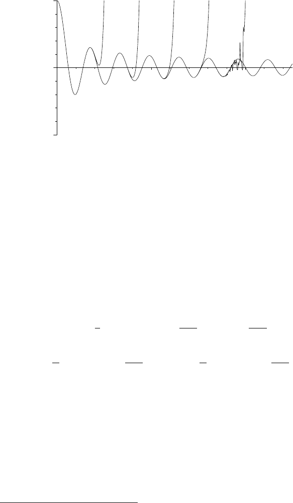
72 CHAPTER 2. APPLICATIONS OF SERIES

–1

20 40

Figure 2.4: Divergent curves from left to right: 20, 40, 60, 80, and 100 terms.

From left to right in Figure 2.4, the divergent curves represent the ﬁnite series

representations of J

for 20, 40, 60, 80, and 100 terms. The non-divergent

oscillatory curve is the inﬁnite series representing the exact J

(x).

2.3 Fourier Series

Consider a single-valued function f(x) deﬁned over the fundamental interval

−L ≤ x ≤ L and satisfying the boundary conditions f (−L)=f(L). If f (x)has

a ﬁnite number of discontinuities and maxima and minima, and



−L

|f(x)| dx

is ﬁnite,

then f(x) can be expanded in the Fourier series ([MW71], [Boa83])

f(x)=

∞



n=1



cos



nπx



+ b

sin



nπx



, (2.8)

with a



−L

f(x)cos



nπx



dx, b



−L

f(x)sin



nπx



dx.

The forms of a

and b

can be derived from Equation (2.8) by noting that

(x) = cos(nπx/L) (or sin(nπx/L)) satisﬁes the orthogonality condition



−L

w(x) y

(x) y

(x) dx =0, for m = n,withw(x) = 1. The identiﬁcation of

w(x) follows on noting that the y

(x) are solutions of y



(x)+(nπ/L)

y(x)=0.

This equation is a Sturm–Liouville ODE, (1.6), with p =1, q =0, w =1, and

λ = −(nπ/L)

.Thea

and b

follow on multiplying (2.8) by cos(nπx/L) (or

sin(nπx/L)), integrating from −L to L, and using the orthogonality condition.

If f(x) is an odd function, that is to say f(−x)=−f(x), then a

= 0 and

=(2/L)



f(x)sin(nπx/L) dx,sof(x) is expressed as a Fourier sine series.

These are suﬃcient, but not necessary, conditions.

2.3. FOURIER SERIES 73

On the other hand, if f(x) is an even function, i.e., f(−x)=f(x), then

=(2/L)



f(x) cos(nπx/L) dx and b

=0, so f(x)isaFourier cosine series.

Since each term in (2.8) is periodic with period 2L,thenf(x +2L)=f(x).

Thus, the Fourier series may either represent an f(x) deﬁned in the fundamental

interval (−L, L), or a periodic f(x) with period 2L for all of x.

When f(x) is deﬁned only in the range 0 to L, it can be written as a Fourier

sine series by including the range to −L to 0 and considering f(x)tobeanodd

function about x = 0. Alternately, it can be written as a Fourier cosine series

by considering f (x) to be an even function about the origin. It may turn out

that one series ﬁts f(x) better than the other for a ﬁnite number of terms.

To this point, the fundamental interval has been taken to be 2L.Thiscan

be easily changed. For example, consider f(t) deﬁned in the range t =0toT

and we want the fundamental interval to be T , not 2T . To accomplish this, set

x = t and L = T/2 in (2.8) and a

and b

and change the range of the integrals

from −T/2 ... T /2to0... T . In this case, the general Fourier expansion becomes

f(t)=

∞



n=1



cos



2nπt



+ b

sin



2nπt



, (2.9)

with a



f(t)cos



2nπt



dt, and b



f(t)sin



2nπt



dt.

Again, this series may be used to represent either a function deﬁned in the

fundamental interval 0 to T or a periodic function whose period is T .

The concept of expanding a function f (x) in terms of sines and cosines can

be extended to other special functions y

(x) satisfying a S-L type equation. If

the y

(x) satisfy the same boundary conditions at a and b as f(x), then

f(x)=



(x), with A



w(x) f(x) y

(x) dx



w(x) y

(x)

. (2.10)

The functions y

(x) are said to form a complete set. Often, they are normalized

so that



w(x) y

(x)

dx= 1. Since they have the orthogonality property, they

then satisfy the orthonormality condition



w(x) y

(x) y

(x) dx = δ

, (2.11)

where δ

,theKronecker delta, is deﬁned by δ

=1 for m =n and 0 for m=n.

As an example of expanding in terms of special functions, the Legendre–

Fourier series (or simply the Legendre series)isgivenby

f(x)=

∞



n=0

(x), with A

(2 n +1)



−1

f(x) P

(x) dx. (2.12)

A mathematical example of this series is given in Recipe 02-3-3.

74 CHAPTER 2. APPLICATIONS OF SERIES

2.3.1 Madeiran Levadas and the Gibb’s Phenomenon

The idealist walks on tiptoe, the materialist on his heels.

Malcolm de Chazal, French writer, (1902–81)

On the island of Madeira, water is transported from the mountains by a net-

work of levadas (irrigation canals) which often cling to the mountain side with

vertigo-inducing drop oﬀs and pass through pitch-black tunnels. This recipe

is inspired by some interesting hikes that I have taken on Madeiran levada re-

taining walls. A levada retaining wall is described by the piecewise function

f =(L + x)/2for−L ≤ x ≤−L/2, f = L/4for−L/2 ≤ x<0, and f =0 for

0 <x≤ L,withL=π. Determine the Fourier series representation of f(x)and

plot it and f together. Calculate the cross-sectional area of the retaining wall

using f(x) and then the Fourier series. Discuss the various results.

To simplify the command entries, let’s set X =πx/L.

restart: X:=Pi*x/L:

Using the inert Sum command, an operator F is formed to calculate the Fourier

series, keeping N terms.

F:=N->a[0]/2+Sum(a[n]*cos(n*X)+b[n]*sin(n*X),n=1..N);

F := N →



n=1

cos(nX)+b

sin(nX)))

The formal expressions for the coeﬃcients are entered using the inert form of

the integral command. In the outputs, X is replaced with πx/L.

a[0]:=(1/L)*Int(f,x=-L..L);



−L

fdx

a[n]:=(1/L)*Int(f*cos(n*X),x=-L..L);



−L

f cos(

nπx

) dx

b[n]:=(1/L)*Int(f*sin(n*X),x=-L..L);



−L

f sin(

nπx

) dx

The value L= π is speciﬁed and the piecewise function f entered.

L:=Pi: f:=piecewise(x<-L/2,(L+x)/2,x<0,L/4,x<L,0);

f :=

⎧

⎪

⎨

⎪

⎩

x<−

x<0

0 x<π

The value of the coeﬃcient a

is obtained.

a[0]:=value(a[0]);

2.3. FOURIER SERIES 75

3 π

The coeﬃcients a

and b

can be simpliﬁed by assuming that n is an integer.

The “type match command” (::) is used in the assumption.

a[n]:=simplify(value(a[n])) assuming n::integer;

:= −

(−1)

− cos(

πn

)

πn

b[n]:=simplify(value(b[n])) assuming n::integer;

:= −

πn+2sin(

πn

)

πn

The Fourier series is generated in FF ,withN =15. (Only the leading terms in

the output are shown here in the text.) You can increase the value of N, but

you might then wish to suppress the very lengthy output by putting a colon on

the end of the command line.

FF:=value(F(15));

FF :=

3 π

cos(x)

−

(π +2)sin(x)

−

cos(2 x)

−

sin(2 x)

cos(3 x)

−

(3 π − 2) sin(3 x)

−

sin(4 x)+

cos(5 x)

+ ···

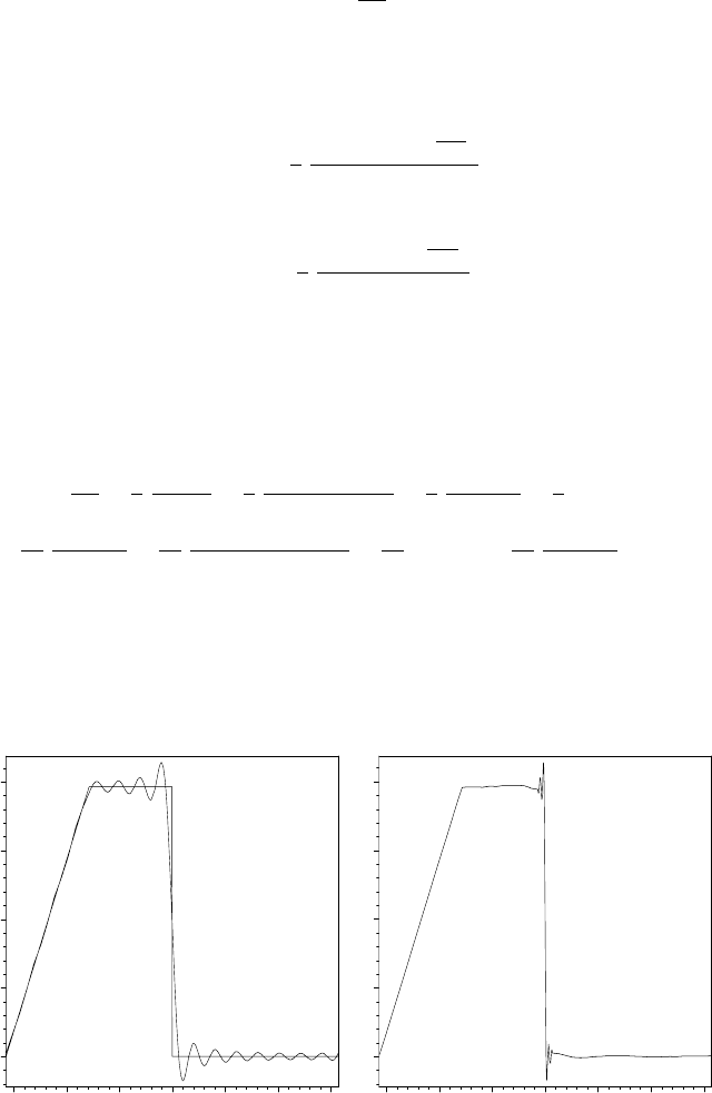
Finally, the function f and the Fourier series FF are plotted over the range

x = −L = −π to x = L = π, being represented by thick blue and red lines. The

resulting picture is shown on the left of Figure 2.5.

plot([f,FF],x=-L..L,color=[blue,red],thickness=2,axes=box);

0.2

0.4

0.6

0.8

–3 –2 –1 0 1 2 3

0.2

0.4

0.6

0.8

–3 –2 –1 0 1 2 3

Figure 2.5: Left: Fourier series for N =15 and f.Right:SeriesforN =100.

76 CHAPTER 2. APPLICATIONS OF SERIES

The Fourier series oscillates around the exact f. The ﬁt can be improved (the

size of the oscillations reduced) by increasing N. The plot on the right of

Figure 2.5 shows the Fourier series result for N = 100. The overshoot in the

vicinity of the step function at x=0 persists, however, no matter how large an

N is chosen. This is called the Gibbs’ phenomenon. Notice also in the left plot

that the Fourier series curve passes approximately through the midpoint of the

step. As N →∞, the Fourier curve will pass exactly though the midpoint, a

general property of Fourier series at step discontinuities.

The exact cross-sectional area of the retaining wall is calculated in Area1 by

integrating f from x =−L= −π to π. The cross-sectional area is also calculated

in Area2 by integrating the Fourier series FF over the same range.

Area1:=int(f,x=-Pi..Pi); Area2:=int(FF,x=-Pi..Pi);

Area1 :=

3 π

Area2 :=

3 π

The two areas are identical. The “wiggles” in the Fourier series about the f

curve exactly cancel. You might like to conﬁrm that this is still true for N = 100.

2.3.2 Sine or Cosine Series?

I see it all perfectly; there are two possible situations – one can either

do this or that. My honest opinion and my friendly advice is this:

do it or do not do it – you will regret both.

Søren Kierkegaard, Danish philosopher, (1813–55)

Consider the function f(x)=x for 0 ≤ x ≤ L/2andf(x)=L − x for

L/2 ≤ x ≤ L,withL = 1. Extending the range to −L ≤ x ≤ L,derivea

Fourier sine series and a cosine series representation of f (x). Plot f(x) and the

two series together and discuss the results.

The value of L is entered and, again for convenience, let’s set X =πx/L.

restart: L:=1: X:=Pi*x/L:

The function f is entered using the piecewise command.

f:=piecewise(x<L/2,x,x<L,L-x);

f :=



xx<

1 − xx<1

An odd function f1 is introduced which is the same as f for 0 ≤ x ≤ L, but is

equal to −f for −L ≤ x ≤ 0. f1 will be used to generate the sine series.

f1:=piecewise(x<-L/2,-(L+x),x<L/2,x,x<L,L-x);

f1 :=

⎧

⎪

⎨

⎪

⎩

−1 − xx<

−1

xx<

1 − xx<1