Francoise J.-P., Naber G.L., Tsun T.S. (editors) Encyclopedia of Mathematical Physics

Подождите немного. Документ загружается.

The critical probability is defined as

:¼p

ðGÞ¼ supfp: ðpÞ¼0g

By definition, when p < p

, the open cluster of the

origin is P

-a.s. finite; hence, all the clusters are also

finite. On the other hand, for p > p

there is a

strictly positive P

-probability that the cluster of the

origin is infinite. Thus, from Kolmogorov’s zero–one

law it follows that

fjCðvÞj ¼ 1 for some v 2Vg¼1 for p > p

Therefore, if the intervals [0, p

) and (p

, 1] are both

nonempty, there is a phase transition at p

Using a so-called Peierls argument it is easy to see

that p

(G) > 0 for any graph G of bounded degree.

On the other hand, Hammersley proved that

) < 1 for bond percolation as soon as d  2,

and a similar argument works for site percolation

and various periodic graphs as well. But for some

graphs G, it is not so easy to show that p

(G) < 1.

One says that the system is in the subcritical (resp.

supercritical) phase if p < p

(resp. p > p

It was one of the most remarkable moments in the

history of percolation when Kesten (1980) proved,

based on results by Harris, Russo, Seymour and

Welsh, that the critical parameter for bond percolation

on Z

is equal to 1/2. Nevertheless, the exact value of

(G) is known only for a handful of graphs, all of

them periodic and two dimensional – see below.

Percolation in Z

The graph on which most of the theory was

originally built is the cubic lattice Z

, and it was

not before the late twentieth century that percola-

tion was seriously considered on other kinds of

graphs (such as Cayley graphs), on which specific

phenomena can appear, such as the coexistence of

multiple infinite clusters for some values of the

parameter p. In this section, the underlying graph is

thus assumed to be Z

for d  2, although most

of the results still hold in the case of a periodic

d-dimensional lattice.

The Subcritical Regime

When p < p

, all open clusters are finite almost

surely. One of the greatest challenges in percolation

theory has been to prove that (p):= E

{jC(v)j}is

finite if p < p

stands for the expectation with

respect to P

). For that one can define another critical

probability as the threshold value for the finiteness of

the expected cluster size of a fixed vertex:

ðGÞ:¼ supfp: ðpÞ< 1g

It was an important step in the development of the

theory to show that p

(G) = p

(G). The fundamental

estimate in the subcritical regime, which is a much

stronger statement than p

(G) = p

(G), is the following:

Theorem 1 (Aize nman and Barsky, Menshikov).

Assume that G is periodic. Then for p < p

there

exist constants 0 < C

, C

< 1, such that

fjCðvÞj  ngC

C

The last statement can be sharpened to a ‘‘local

limit theorem’’ with the help of a subadditivity

argument: for each p < p

, there exists a constant

0 < C

(p) < 1, such that

lim

n!1



log P

fjCðvÞj ¼ ng¼C

ðpÞ

The Supercritical Regime

Once an infinite open cluster exists, it is natural to

ask how it looks like, and how many infinite open

clusters exist. It was shown by Newman and Schul-

man that for periodic graphs, for each p, exactly one

of the following three situations prevails: if N 2

[ {1} is the number of infinite open clusters, then

(N = 0) = 1, or P

(N = 1) = 1, or P

(N = 1) = 1.

Aizenman, Kesten, and Newman showed that the

third case is impossible on Z

. By now several

proofs exist, perhaps the most elegant of which is

due to Burton and Keane, who prove that indeed

there cannot be infinitely many infinite open clusters

on an y amenable graph. However, there are some

graphs, such as regular trees, on which coexistence

of several infinite clusters is possible.

The geometry of the infini te open cluster can be

explored in some depth by studying the behavior of

a random walk on it. When d = 2, the random walk

is recurrent, and when d  3 is a.s. transient. In all

dimensions d  2, the walk behaves diffusively, and

the ‘‘central limit theorem’’ and the ‘‘invariance

principle’’ were established in both the annealed and

quenched cases.

Wulff droplets In the supercritical regime, aside

from the infinite open cluster, the configuration

contains finite clusters of arbitrary large sizes. These

large finite open clusters can be thought of as droplets

swimming in the areas surrounded by an infinite open

cluster. The presence at a particular location of a large

finite cluster is an event of low probability, namely, on

, d  2, for p > p

, there exist positive constants

0 < C

(p), C

(p) < 1,suchthat

ðpÞ

ðd1Þ=d

log P

fjCðvÞj ¼ ngC

ðpÞ

22 Percolation Theory

for all large n. This estimate is based on the fact that

the occurrence of a large finite cluster is due to a

surface effect. The typical structure of the large

finite cluster is described by the following theorem:

Theorem 2 Let d  2, and p > p

. There exists a

bounded, closed, convex subset W of R

containing

the origin, called the normalized Wulff crystal of

the Bernoulli percolation model, such that, under the

conditional probability P

{jn

jC(0)j< 1}, the

random measure

x2Cð0Þ



x=n

(where 

denotes a Dirac mass at x) converges

weakly in probability toward the random measure

(p)1

(x  M)dx (where M is the rescaled center of

mass of the cluster C(0)). The deviation probabilities

behave as exp{cn

d1

}(i.e., they exhibit large

deviations of surface order; in dimensions 4 and

more it holds up to re-centering).

This result was proved in dimension 2 by Alexander

et al. (1990), and in dimensions 3 and more by Cerf

(2000).

Percolation Near the Critical Point

Percolation in Slabs The main macroscopic obser-

vable in percolation is (p), which is positive above

, 0 below p

, and continuous on [0, 1]n{p

Continuity at p

is an open question in the general

case; it is known to hold in two dimensions

(cf. below) and in high enough dimension (at the

moment d  19 though the value of the critical

dimension is believed to be 6) using lace expansion

methods. The conjecture that (p

) = 0for3d 18

remains one of the major open problems.

Efforts to prove that led to some interesting and

important results. Barsky, Grimmett, and Newman

solved the question in the half-space case, and simulta-

neously showed that the slab percolation and half-space

percolation thresholds coincide. This was complemen-

ted by Grimmett and Marstrand showing that

ðslabÞ¼p

ðZ

Critical exponents In the subcritical regime, expo-

nential decay of the correlation indicates that there

is a finite correlation length (p) associated to the

system, and defined (up to constants) by the relation

ð0 $ nxÞexp 

n’ðxÞ

ðpÞ



where ’ is bounded on the unit sphere (this is known

as Ornstein–Zernike decay). The phase transition can

then also be defined in terms of the divergence of the

correlation length, leading again to the same value for

; the behavior at or near the critical point then has no

finite characteristic length, and gives rise to scaling

exponents (conjecturally in most cases).

The most usual critical exponents are defined as

follows, if (p) is the percolation probability, C the

cluster of the origin, and (p) the correlation length:

½jCj

1

jp  p

1

ðpÞðp  p





ðpÞ:¼E

½jCj1

jCj<1

jp  p



½jCj¼nn

11=

½x 2 Cjxj

2d

ðpÞjp  p



½diamðCÞ¼nn

11=

½jCj

kþ1

jCj<1



½jCj

jCj<1



jp  p



These exponents are all expected to be universal,

that is, to depend only on the dimension of the

lattice, although this is not well understood at the

mathematical level; the following scaling relations

between the exponents are believed to hold:

2   ¼  þ 2 ¼ ð þ 1Þ;  ¼ ;  ¼ ð2  Þ

In addition, in dimensions up to d

= 6, two

additional hyperscaling relations involving d are

strongly conjectured to hold:

d ¼  þ 1; d ¼ 2  

while above d

the exponents are believed to take

their mean-field value, that is, the ones they have for

percolation on a regular tree:

 ¼1;¼ 1 ;¼ 1;¼ 2

 ¼ 0;¼

;¼

;  ¼ 2

Not much is known rigorously on critical expo-

nents in the general case. Hara and Slade (1990)

proved that mean field behavior does happen above

dimension 19, and the proof can likely be extended

to treat the case d  7. In the two-dimensional case

on the other hand, Kesten (1987) showed that,

assuming that the exponents  and  exist, then so

do , , , and , and they satisfy the scaling and

hyperscaling relations where they appear.

The incipient infinite cluster When studying long-

range properties of a critical model, it is useful to

have an object which is infinite at criticality, and

such is not the case for percolation clusters. There

are two ways to condition the cluster of the origin to

Percolation Theory 23

be infinite when p = p

: The first one is to condition

it to have diameter at least n (which happens with

positive probability) and take a limit in distribution

as n goes to infinity; the second one is to consider

the model for parameter p > p

, condition the

cluster of 0 to be infinite (w hich happens with

positive probability) and take a limit in distribution

as p goes to p

. The limit is the same in both cases; it

is known as the incipient infinite cluster.

As in the supercritical regime, the structure of the

cluster can be investigated by studyi ng the behavior

of a random walk on it, as was suggested by de

Gennes; Kesten proved that in two dimensions, the

random walk on the incipient infinite cluster is

subdiffusive, that is, the mean square displacement

after n steps behaves as n

1"

for some ">0.

The construction of the incipient infinite cluster

was done by Kesten (1986) in two dimensions, and a

similar construction was performed recently in high

dimension by van der Hofstad and Jarai (20 04).

Percolation in Two Dimensions

As is the case for several other models of statistical

physics, percolation exhibits many specific properties

when considered on a two-dimensional lattice: duality

arguments allow for the computation of p

in some

cases, and for the derivation of a priori bounds for the

probability of crossing events at or near the critical

point, leading to the fact that (p

) = 0. On another

front, the scaling limit of critical site percolation on the

two-dimensional triangular lattice can be described in

terms of Stochastic Loewner evolutions (SLE) processes.

Duality, Exact Computations, and RSW Theory

Given a planar latti ce L, define two associated

graphs as follows. The dual lattice L

has one vertex

for each face of the original lattice, and an edge

between two vertices if and only if the correspond-

ing faces of L share an edge. The star graph L



obtained by adding to L an edge between any two

vertices belonging to the same face (L



is not planar

in general; (L, L



) is commonly known as a

matching pair). Then, a result of Kesten is that,

under suitable technical conditions,

bond

ðLÞ þ p

bond

ðL

Þ¼p

site

ðLÞ þ p

site

ðL



Þ¼1

Two cases are of particular importance: the lattice

is isomorphic to its dual; the triangular lattice T

is its own star graph. It follows that

bond

ðZ

Þ¼p

site

ðT Þ¼

The only other critical parameters that are known

exactly are p

bond

(T ) = 2 sin (=18) (and hence also

bond

for T

, i.e., the hexagonal lattice) and p

bond

for

the bow-tie lattice which is a root of the equation

 6p

þ 6p

þ p  1 = 0. The value of the critical

parameter for site percolation on Z

might, on the

other hand, never be known; it is even possible that

it is ‘‘just a number’’ without any other signification.

Still using duality, one can prove that the

probability, for bond percolation on the square

lattice with parameter p = 1=2, that there is a

connected component crossing an (n þ 1)  n rec-

tangle in the longer direction is exact ly equal to 1/2.

This and clever arguments involving the symmetry

of the lattice lead to the following result, proved

independently by Russo and by Seymour and Welsh

and known as the RSW theorem:

Theorem 3 (Russo 1978, Seymour and Welsh 1978).

For every a, b > 0 there exist >0 and n

> 0 such

that for every n > n

, the probability that there is a

cluster crossing an bnacbnbc rectangle in the first

direction is greater than .

The most direct consequence of this estimate is that

the probability that there is a cluster going around an

annulus of a given modulus is bounded below

independently of the size of the annulus; in particular,

almost surely there is some annulus around 0 in

which this happens, and that is what allows to prove

that (p

) = 0 for bond percolation on Z

(Figure 2).

The Scaling Limit

RSW-type estimates give positive evidence that a

scaling limit of the model should exist; it is indeed

essentially sufficient to show convergence of the

crossing probabilities to a nontrivial limit as n goes

to infinity. The limit, which should depend only on

the ratio a/b, was predicted by Cardy using con-

formal field theory methods. A celebrated result of

Smirnov is the proof of Cardy’s formula in the case of

site percolation on the triangular lattice T :

Theorem 4 (Smirnov (2001)). Let  be a simply

connected domain of the plane with four points a , b ,

c, d (in that order) marked on its boundary. For

every >0, consider a critical site-percolation

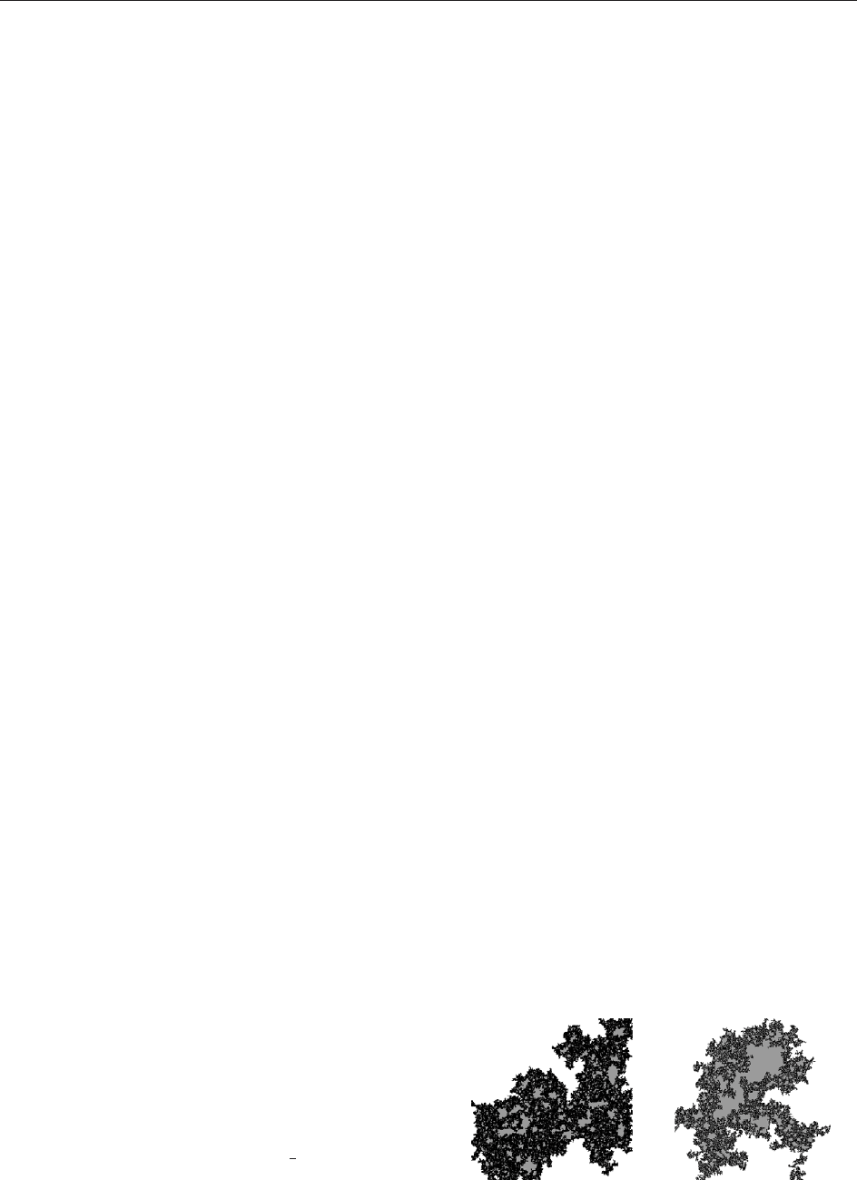
Figure 2 Two large critical percolation clusters in a box of the

square lattice (first: bond percolation, second: site percolation).

24 Percolation Theory

model on the intersection of  with T and let



(ab, cd; ) be the probability that it contains a

cluster connecting the arcs ab and cd. Then:

(i) f



(ab, cd; ) has a limit f

(ab, cd; ) as  !0;

(ii) the limit is conformally invariant, in the

following sense: if  is a conformal map from

 to some other domain 

=(), and maps

atoa

, btob

, ctoc

and d to d

, then

(ab, cd; ) = f

, c

; 

); and

(iii) in the particular case when  is an equilateral

triangle of side length 1 with vertices a, b and c,

and if d is on (ca) at distance x 2 (0, 1) from c,

then f

(ab, cd; ) = x.

Point (iii) in particular is essential since it allows

us to compute the limiting crossing probabilities in

any conformal rectangle. In the original work of

Cardy, he made his prediction in the case of a

rectangle, for which the limit involves hypergeo-

metric functions; the rem ark that the equilateral

triangle gives rise to nicer formulae is originally due

to Carleson.

To precisely state the convergence of percolation

to its scaling limit, define the random curve known

as the percolation exploration path (see Figure 3)as

follows: In the upper half-plane, consider a site-

percolation model on a portion of the triangular

lattice and impose the boundary conditions that on

the negative real half-line all the sites are open,

while on the other half-line the sites are closed. The

exploration curve is then the common boundary of

the open cluster spanning from the negative half-

line, and the closed cluster spanning from the

positive half-line; it is an infinite, self-avoiding

random curve in the upper half-plan e.

As the mesh of the lattice goes to 0, the exploration

curve then converges in distribution to the trace of an

SLE process, as introduced by Schramm, with

parameter  = 6 – see Figure 4. The limiting curve is

not simple anymore (which corresponds to the

existence of pivotal sites on large critical percolation

clusters), and it has Hausdorff dimension 7/4. For

more details on SLE processes, see, for example, the

related entry in the present volume.

As an application of this convergence result, one

can prove that the critical exponents described in the

previous section do exist (still in the case of the

triangular lattice), and compute their exact values,

except for , which is still listed here for

completeness:

 ¼



; ¼

; ¼

; ¼

 ¼

; ¼

;¼

;  ¼

These exponents are expected to be universal, in the

sense that they should be the same for percolation

on any two-dimensional lattice; but at the time of

this writing, this phenomenon is far from being

understood on a mathematical level.

The rigorous derivation of the critical exponents

for percolation is due to Smirnov and Werner

(2001); the dimension of the limiting curve was

obtained by Beffara (2004).

Other Lattices and Percolative Systems

Some modifications or generalizations of standard

Bernoulli percolation on Z

exhibit an interesting

behavior and as such provide some insight into the

original process as well; there are too many

mathematical objects which can be argued to be

percolative in some sense to give a full account of all

Figure 3 A percolation exploration path. Figure courtesy

Schramm O (2000) Scaling limits of loop-erased random walks

and uniform spanning trees. Israel Journal of Mathematics 118:

221–228.

Figure 4 An SLE process with parameter  = 6 (infinite time,

with the driving process stopped at time 1).

Percolation Theory 25

of them, so the following list is somewhat arbitrary

and by no means complete.

Percolation on Nonamenable Graphs

The first modification of the model one can think of

is to modi fy the underlying graph and move away

from the cubic lattice; phase transition still occurs,

and the main difference is the possibility for

infinitely many infinite clusters to coexist. On a

regular tree, such is the case whenever p 2 (p

, 1),

the first nontrivial example was produced by

Grimmett and Newman as the product of Z by a

tree: there, for some values of p the infinite cluster is

unique, while for others there is coexistence of

infinitely many of them. The corresponding defini-

tion, due to Benjamini and Schramm, is then the

following: if N is as above the number of infinite

open clusters,

:¼inf p : P

ðN ¼ 1Þ¼1



 p

The main question is then to characterize graphs on

which 0 < p

< p

< 1.

A wide class of interesting graphs is that of Cayley

graphs of infinite, finitely generated groups. There,

by a simultaneous result by Ha¨ ggstro¨ m and Peres

and by Schonmann, for every p 2 (p

, p

) there are

-a.s. infinitely many infinite cluster, while for

every p 2 (p

, 1] there is only one – note that this

does not follow from the definition since new

infinite components could appear when p is

increased. It is conjectured that p

< p

for any

Cayley graph of a nonamenable group (and more

generally for any quasitransitive graph with positive

Cheeger constant), and a result by Pak and

Smirnova is that every infinite, finitely generated,

nonamenable group has a Cayley graph on which

< p

; this is then expected not to depend on the

choice of generators. In the general case, it was recently

proved by Gaboriau that if the graph G is unimodular,

transitive, locally finite, and supports nonconstant

harmonic Dirichlet functions (i.e., harmonic functions

whose gradient is in ‘

), then indeed p

(G) < p

(G).

For referenc e a nd further r eading on the t opic,

the reader is advised to refer to the review paper by

Benjamini and Schramm (1996), the lecture notes

of Peres (1999), and the more recent article of

Gaboriau (2005).

Gradient Percolation

Another possible modification of the original model

is to allow the parameter p to depend on the

location; the porous medium may for instance have

been created by some kind of erosion, so that there

will be more open edges on one side of a given

domain than on the other. If p still varies smoothly,

then one expects some regions to look subcritical

and others to look supercritical, with interesting

behavior in the vicinity of the critical level set

{p = p

}. This pa rticular model was introduced by

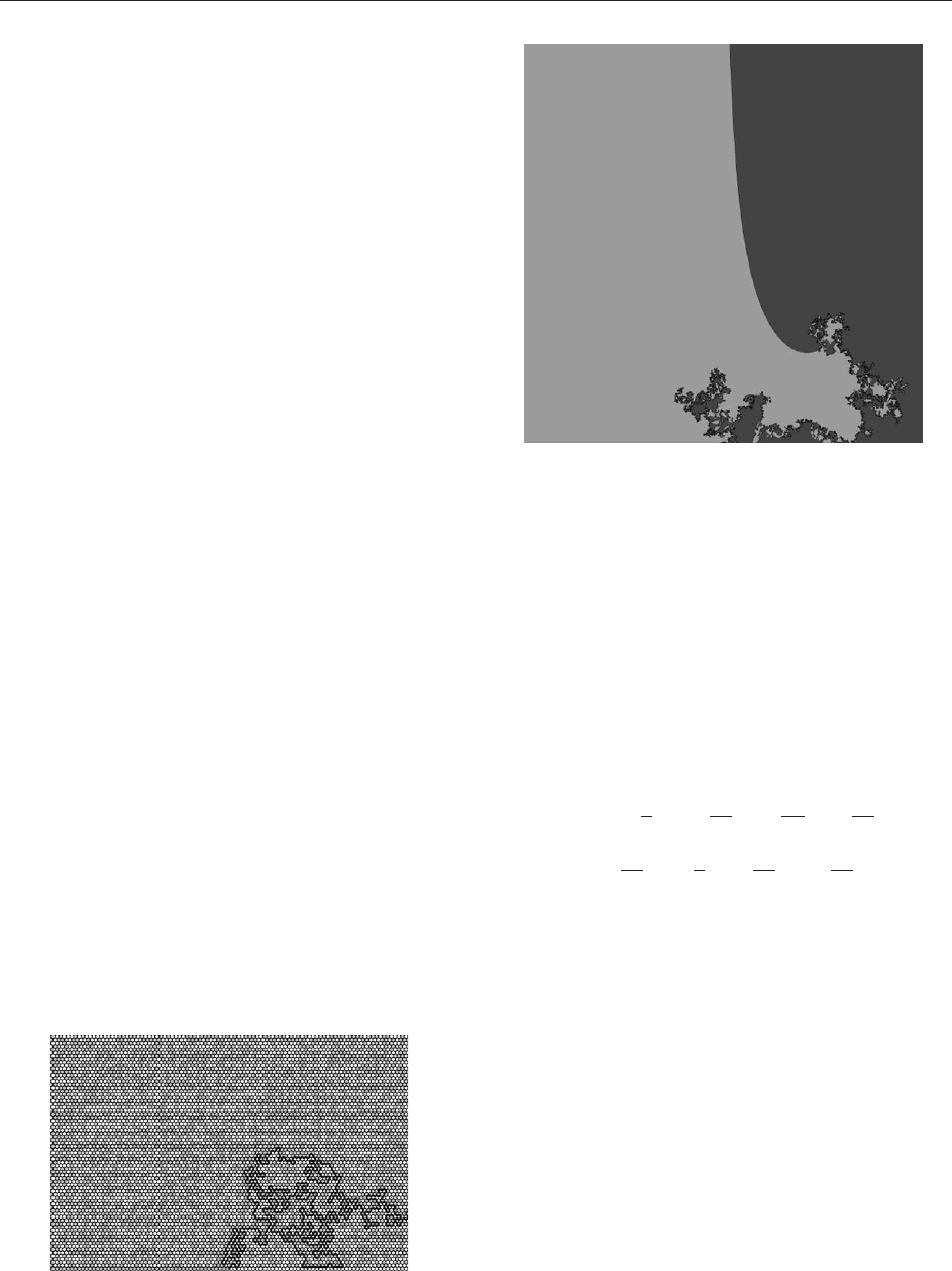
Sapoval et al. (1978) under the name of gradient

percolation (see Figure 5).

The control of the model away from the critical

zone is essentially the same as for usual Bernoulli

percolation, the main question being how to

estimate the width of the phase transition. The

main idea is then the same as in scaling theory: if the

distance between a point v and the critical level set is

less than the correlation length for parameter p(v),

then v is in the phase transition domain. This of

course makes sense only asymptotically, say in a

large n  n square with p(x, y) = 1  y=n as is the

case in the figure: the transition then is expected to

have width of order n

for some exponent a > 0.

First-Passage Percolation

First-passage percolation (also known as Eden or

Richardson model) was introduced by Hammersley

and Welsh (1965) as a time-dependent model for the

passage of fluid through a porous medium. To define

the model, with each edge e 2E(Z

)isassociateda

random variable T(e), which can be interpreted as

being the time required for fluid to flow along e.The

T(e) are assumed to be independent non-negative

random variables having common distribution F.For

any path  we define the passage time T()of as

TðÞ:¼

e2

TðeÞ

Figure 5 Gradient percolation in a square. In black is the

cluster spanning from the bottom side of the square.

26 Percolation Theory

The first passage time a(x, y) between vertices x and

y is given by

aðx; yÞ¼inffTðÞ:  a path from x to yg

and we can define

WðtÞ:¼fx 2 Z

: að0; xÞtg

the set of vertices reached by the liquid by time t.It

turns out that W(t) grows approximately linearly as

time passes, and that there exists a nonrandom limit

set B such that either B is compact and

ð1  "ÞB 

WðtÞð1 þ "ÞB; eventually a:s:

for all >0, or B = R

, and

fx 2 R

: jxjKg

WðtÞ; eventually a:s:

for all K > 0. Here

W(t) = {z þ [ 1=2, 1=2]

z 2 W(t)}.

Studies of first-passage percolation brought

many fascinating discoveries, including Kingman’s

celebrated subadditive ergodic theorem. In recent

years interest has been focused on study of

fluctuations of the set

W(t)forlarget. In spite of

huge effort and some partial results achieved, it

still remains a major task to establish rigorously

conjectures predicted by Kardar–Parisi–Zhang the-

ory about shape fluctuations in first passage

percolation.

Contact Processes

Introduced by Harris and conceived with biological

interpretation, the contact process on Z

is a

continuous-time process taking value s in the space

of subsets of Z

. It is informally described as

follows: particles are distri buted in Z

in such a

way that each site is either empty or occupied by

one particle. The evolution is Markovian: each

particle disappea rs after an exponential time of

parameter 1, independently from the others; at any

time, each particle has a possibility to create a new

particle at any of its empty neighboring sites, and

does so with rate >0, independently of everything

else.

The question is then whether, starting from a

finite population, the process will die out in finite

time or whether it will survive forever with positive

probability. The outcome will depend on the value

of , and there is a critical va lue 

, such that for

  

process dies out, while for >

indeed

there is survival, and in this case the shape of the

population obeys a shape theorem similar to that of

first-passage percolatio n.

The analogy with percolation is strong, the

corresponding percolative picture being the follow-

ing: in Z

dþ1

, each edge is open with probability p 2

(0, 1), and the question is whether there exists an

infinite oriented path  (i.e., a path along which the

sum of the coordinates is increasing), composed of

open edges. Once again, there is a critical parameter

customarily denoted by p

, at which no such path

exists (compare this to the open question of the

continuity of the function  at p

in dimensions

3  d  18). This variation of percolation lies in a

different universality class than the usual Bernoulli

model.

Invasion Percolation

Let X(e):e 2E be independent random variables

indexed by the edge set E of Z

, d  2, each

having uniform distribution in [0, 1]. One con-

structs a sequence C = {C

, i 1} of random

connected subgraphs of the lattice in the

following iterative way: the graph C

contains

only the origin. Having defined C

, one obtains

iþ1

by adding to C

an edge e

iþ1

(with its outer

lying end-vertex), chosen from the outer edge

boundary of C

so as to minimize X(e

iþ1

). Still

very little is known about the behavior of this

process.

An interesting observation, relating (p

) of usual

percolation with the invasion dynamics, comes from

CM Newman:

ðp

Þ¼0 , Pfx 2 Cg!0asjxj!1

Further Remarks

For a much more in-depth review of percolation on

lattices and the mathematical methods involved in

its study, and for the proofs of most of the results we

could only point at, we refer the reader to the

standard book of Grimmett (1999); another excel-

lent general reference, and the only place to find

some of the technical graph-theoretical details

involved, is the book of Kesten (1982). More

information in the case of graphs that are not

lattices can be found in the lecture notes of Peres

(1999).

For curiosity, the reader can refer to the first

mention of a problem close to percolation, in the

problem section of the first volume of the American

Mathematical Monthly (problem 5, June 1894,

submitted by D V Wood).

See also: Determinantal Random Fields; Stochastic

Loewner Evolutions; Two-Dimensional Ising Model; Wulff

Droplets.

Percolation Theory 27

Further Reading

Alexander K, Chayes JT, and Chayes L (1990) The Wulff

construction and asymptotics of the finite cluster distribution

for two-dimensional Bernoulli percolation. Communications

in Mathematical Physics 131: 1–50.

Beffara V (2004) Hausdorff dimensions for SLE

. Annals of

Probability 32: 2606–2629.

Benjamini I and Schramm O (1996) Percolation beyond Z

, many

questions and a few answers. Electronic Communications in

Probability 1(8): 71–82 (electronic).

Broadbent SR and Hammersley JM (1957) Percolation processes,

I and II. Mathematical Proceedings of the Cambridge

Mathematical Society 53, pp. 629–645.

Cerf R (2000) Large deviations for three dimensional supercritical

percolation. Aste´risque, SMF vol. 267.

Gaboriau D (2005) Invariant percolation and harmonic Dirichlet

functions. Geometric and Functional Analysis (in print).

Grimmett G (1999) Percolation. Grundlehren der Mathematischen

Wissenschaften, 2nd edn, vol. 321. Berlin: Springer.

Hammersley JM and Welsh DJA (1965) First-passage percolation,

subadditive processes, stochastic networks, and generalized

renewal theory. In: Proc. Internat. Res. Semin,Statist.Lab.,

Univ. California, Berkeley, CA, pp. 61–110. New York: Springer.

Hara T and Slade G (1990) Mean-field critical behaviour for

percolation in high dimensions. Communications in Mathe-

matical Physics 128: 333–391.

Kesten H (1980) The critical probability of bond percolation on

the square lattice equals 1/2. Communications in Mathema-

tical Physics 74: 41–59.

Kesten H (1982) Percolation Theory for Mathematicians, Pro-

gress in Probability and Statistics, vol. 2. Boston, MA:

Birkha¨user.

Kesten H (1986) The incipient infinite cluster in two-dimensional

percolation. Probability Theory and Related Fields 73:

369–394.

Kesten H (1987) Scaling relations for 2D-percolation. Commu-

nications in Mathematical Physics 109: 109–156.

Peres Y (1999) Probability on Trees: An Introductory Climb,

Lectures on Probability Theory and Statistics (Saint-Flour,

1997), Lecture Notes in Math, vol. 1717, pp. 193–280. Berlin:

Springer.

Russo L (1978) A note on percolation. Zeitschift fu¨r Wahrschein-

lichkeitstheorie und Verwandte Gebiete 43: 39–48.

Sapoval B, Rosso M, and Gouyet J (1985) The fractal nature of a

diffusion front and the relation to percolation. Journal de

Physique Lettres 46: L146–L156.

Seymour PD and Welsh DJA (1978) Percolation probabilities on the

square lattice. Annals of Discrete Mathematics 3: 227–245.

Smirnov S (2001) Critical percolation in the plane: conformal

invariance, Cardy’s formula, scaling limits. Comptes-rendus de

l’Acade´mie des Sciences de Paris, Se´rie I Mathe´matiques 333:

239–244.

Smirnov S and Werner W (2001) Critical exponents for two-

dimensional percolation. Mathematical Research Letters 8:

729–744.

van der Hofstad R and Ja´rai AA (2004) The incipient infinite

cluster for high-dimensional unoriented percolation. Journal

of Statistical Physics 114: 625–663.

Perturbation Theory and Its Techniques

R J Szabo, Heriot-Watt University, Edinburgh, UK

Introduction

There are several equivalent formulations of the

problem of quantizing an interacting field theory.

The list includes canonical quantization, path-

integral (or functional) techniques, stochastic

quantization, ‘‘unified’’ methods such as the

Batalin–Vilkovisky formalism, and techniques

based on the realizations of field theories as low-

energy limits of string theory. The problem of

obtaining an exact nonperturbative description of a

given quantum field theory is most often a very

difficult one. Perturbative techniques, on the other

hand, are abundant, and common to all of the

quantization methods mentioned above is that they

admit particle interpretations in this formalism.

The basic physical quantities that one wishes to

calculate in a relativistic (d þ 1)-dimensional quan-

tum field theory are the S-matrix elements

out

ðtÞj

ðtÞi

½1

between in and out states at large positive time t.

The scattering operator S is then defined by writing

[1] in terms of initial free-particle (descriptor) states as

¼: h

ð0ÞjSj

ð0Þi ½2

Suppose that the Hamiltonian of the given field

theory can be written as H = H

þ H

, where H

the free part and H

the interaction Hamiltonian.

The time evolutions of the in and out states are

governed by the total Hamiltonian H. They can be

expressed in terms of descriptor states which evolve

in time with H

in the interaction picture and

correspond to free-particle states. This leads to the

Dyson formula

S ¼ T exp i

1

dtH

ðtÞ



½3

where T denotes time ordering and H

(t) =

int

(x, t) is the interaction Hamiltonian in the

interaction picture, with H

int

(x, t) the inte raction

Hamiltonian density, which deals with essentially

free fields. This formula expresses S in terms of

interaction-picture operators acting on free-particle

states in [2] and is the first step towards Feynman

perturbation theory.

28 Perturbation Theory and Its Techniques

For many analytic investigations, such as those

which arise in renormalization theory, one is

interested instead in the Green’s functions of the

quantum field theory, which measure the response

of the system to an external perturbation. For

definiteness, let us consider a free real scalar field

theory in d þ 1 dimensions with Lagrangian

density

L¼



@



 



þL

int

½4

where L

int

is the interaction Lagrangian density

which we assume has no derivative terms. The

interaction Hamiltonian density is then given by

int

= L

int

. Introducing a real scalar source J(x),

we define the normalized ‘‘partition function’’

through the vacuum expectation values,

Z½J¼

h0jS½Jj0i

h0jS½0j0i

½5

where j0i is the normalized perturbative vacuum

state of the quantum field theory given by (4)

(defined to be destroyed by all field annihilation

operators), and

S½J¼T exp i

dþ1

xðL

int

þ JðxÞðxÞÞ



½6

from the Dyson formula. This partition function is

the generating functional for all Green’s functions

of the quantum field theory, which are obtained

from [5] by taking functional derivatives with

respect to the source and then setting J(x) = 0.

Explicitly, in a formal Taylor series expansion in J

one has

Z½J¼

n¼0

i¼1

dþ1

Jðx

ÞG

ðnÞ

ðx

; ...; x

Þ½7

whose coefficients are the Green’s functions

ðnÞ

ðx

;...;x

:¼

h0jT½exp i

dþ1

int



ðx

Þðx

Þj0i

h0jTexp i

dþ1

int



j0i

½8

It is customary to work in momentum space by

introducing the Fourier transforms

JðkÞ¼

dþ1

x e

ikx

JðxÞ

ðnÞ

ðk

; ...; k

i¼1

dþ1

x

ðnÞ

ðx

; ...; x

½9

in terms of which the expansion [7] reads

Z½ J ¼

n¼0

i¼1

dþ1

ð2Þ

dþ1

Jðk



ðnÞ

ðk

; ...; k

Þ½10

The generating functional [10] can be written as a sum

of Feynman diagrams with source insertions. Dia-

grammatically, the Green’s function is an infinite series

of graphs which can be represented symbolically as

(n)

, . . . ,k

) =

½11

where the n external lines denote the source

insertions of momenta k

and the bubble denotes

the sum over all Feynman diagrams constructed

from the interaction vertices of L

int

This procedure is, however, rather formal in the way

that we have presented it, for a variety of reasons. First

of all, by Haag’s theorem, it follows that the interaction

representation of a quantum field theory does not exist

unless a cutoff regularization is introduced into the

interaction term in the Lagrangian density (this

regularization is described explicitly below). The

addition of this term breaks translation covariance.

This problem can be remedied via a different definition

of the regularized Green’s functions, as we discuss

below. Furthermore, the perturbation series of a

quantum field theory is typically divergent. The

expansion into graphs is, at best, an asymptotic series

which is Borel summable. These shortcomings will not

be emphasized any further in this article. Some

mathematically rigorous approaches to perturbative

quantum field theory can be found in the bibliography.

The Green’s functions can also be used to describe

scattering amplitudes, but there are two important

differences between the graphs [11] and those which

appear in scattering theory. In the present case,

external lines carry propagators, that is, the free-

field Green’s functions

ðx  yÞ¼ 0TðxÞðyÞ½

¼ x & þ m



1



dþ1

ð2Þ

dþ1

 m

þ i

ipðxyÞ

½12

where  !0

regulates the mass shell contributions,

and their momenta k

are off-shell in general

6¼m

). By the LSZ theorem, the S-matrix element

Perturbation Theory and Its Techniques 29

is then given by the multiple on-shell residue of the

Green’s function in momentum space as

; ...; k

S  1

; ...; k



¼ lim

;...;k

i¼1

ﬃﬃﬃﬃ

 m



j¼1

ﬃﬃﬃﬃ

 m





ðnþmÞ

k

; ...; k

; k

; ...; k



½13

where ic

,ic

are the residues of the corresponding

particle poles in the exact two-point Green’s

function.

This article deals with the formal development

and computation of perturbative scattering ampli-

tudes in relativistic quantum field theory, along the

lines outlined above. Initially we deal only with real

scalar field theories of the sort [4] in order to

illustrate the concepts and technical tools in as

simple and concise a fashion as possible. These

techniques are common to most quantum field

theories. Fermions and gauge theories are then

separately treated afterwards, focusing on the

methods which are particular to them.

Diagrammatics

The pinnacle of perturbation theory is the technique

of Feynman diagrams. Here we develop the basic

machinery in a quite general setting and use it to

analyze some generic features of the terms compris-

ing the perturbation series.

Wick’s Theorem

The Green’s functions [8] are defined in terms of

vacuum expectation values of time-ordered products

of the scalar field (x) at different spacetime points.

Wick’s theorem expresses such products in terms of

normal-ordered products, defined by placing each

field creation operator to the right of each field

annihilation operator, and in terms of two-point

Green’s functions [12] of the free-field theory

(propagators). The consequence of this theorem is

the Haffnian formula

0Tðx

Þðx

Þ½

n ¼ 2k  1

2S

i¼1

0Tð x

ð2i1Þ

Þðx

ð2iÞ







n ¼ 2k

½14

The formal Taylor series expansion of the

scattering operator S may now be succinctly

summarized into a diagrammatic notation by

using Wick’s theorem. For each spacetime integra-

tion

dþ1

we introduce a vertex with label i,

and from each vertex there emanate some lines

corresponding to field insertions at the point x

If the operators represented by two lines appear in

a two-point function according to [14], that is, they

are contracted, then these two lines are connected

together. The S operator is then represented as a

sum over all such Wick diagrams, bearing in mind

that topologically equivalent diagrams correspond

to the same term in S. Two diagrams are said to

have the same pattern if they differ only by a

permutation of their vertices. For any diagram D

with n(D) vertices, the number of ways of inter-

changing vertices is n(D)!. The number of diagrams

per pattern is always less than this number. The

symmetry number S(D)ofD is the number of

permutations of vertices that give the same dia-

gram. The number of diagrams with the pattern of

D is then n(D)!=S(D).

In a given pattern, we write the contribution to S

of a single diagram D as

nðDÞ!

:ðDÞ:

where the combinatorial factor comes from

the Taylor expansion of S, the large colons

denote normal ordering of quantum operators,

and : (D): contains spacetime integrals over nor-

mal-ordered products of the fields. Then all

diagrams with the pattern of D contribute :(D) :

=S(D)toS. Only the connected diagrams D

, r 2 N

(those in which every vertex is connected to every

other vertex) contribute and we can write the

scattering operator in a simple form which

eliminates contributions from all disconnected dia-

grams as

S ¼: exp

r¼1

ðD

SðD

: ½15

Feynman Rules

Feynman diagrams in momentum space are

defined from the Wick diagrams above by drop-

ping the labels on vertices (and also the symmetry

factors S(D)

1

), and by labeling the external lines

by the momenta of the initial and final particles

that the corresponding field operators annihilate.

In a spacetime interpretation, external lines

30 Perturbation Theory and Its Techniques

represent on-shell physical particles while internal

lines of the graph represent off-shell virtual

particles (k

6¼ m

). Physical particles interact

via the exchange of virtual particles. An arbitrary

diagram is then calculated via the Feynman rules:

ig (2π)

d +1

(d +1)

+ · · · + p

)

d +1

(2π)

d +1

–

+ i

½16

for a monomial interaction L

int

= (g=n!)

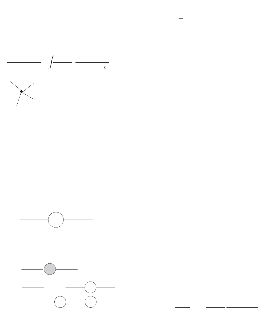
Irreducible Green’s Functions

A one-particle irreducible (1PI) or proper Green’s

function is given by a sum of diagrams in which

each diagram cannot be separated by cutting one

internal line. In momentum space, it is defined

without the overall momentum conservation delta-

function factors and without propagators on exter-

nal lines. For example, the two particle 1PI Green’s

function

1PI

: ∑(k)

½17

is called the self-energy. If G(k)isthecomplete

two-point function in momentum space, then one

has

–

∑(k)

G(k) :

1PI

. . .

½18

and thus it suffices to calculate only 1PI diagrams.

The 1PI effective action, defined by the Legendre

transformation []:= ilnZ[J] 

dþ1

xJ(x)(x)

of [5], is the generating functional for proper vertex

functions and it can be represented as a functional of

only the vacuum expectation value of the field ,

that is, its classical value. In the semiclassical (WKB)

approximation, the one-loop effective action is

given by

½¼S½þ

ih

Tr ln 1 þ V

½ðÞþOðh

¼ S½þih

n¼1

ð1Þ



i¼1

dþ1

ðx

 x

iþ1

ÞV

ðx

iþ1

Þ½

þ Oðh

Þ½19

wherewehavedenotedS[] =

dþ1

xL and

V[] = L

int

, and for each term in the infinite

series we define x

nþ1

:= x

. The first term in [19]

is the classical contribution and it can be

represented in terms of connected tree diagrams.

The second term is the sum of contributions of

one-loop diagrams constructed from n propaga-

tors i(x  y)andn vertices iV

[]. The

expansion may be carried out to all orders in

terms of connected Feynman diagrams, and the

result of the above Legendre transformation is to

select only the one-particle irreducible diagrams

and to replace the classical value of  by an

arbitrary argument. All information about the

quantum field theory is encoded in this effective

action.

Parametric Representation

Consider an arbitrary proper Feynman diagram

D with n internal lines and v vertices. The

number, ‘, of independent loops in the diagram

is the number of independent internal momenta in

D when conservation laws at each vertex have

been taken into account, and it is given by ‘ = n þ

1  v. There is an independent momentum inte-

gration variable k

for each loop, and a propa-

gator for each internal line as in [16].The

contribution of D to a proper Green’s function

with r incoming external momenta p

,with

i = 1

= 0, is given by

ðpÞ¼

VðDÞ

SðDÞ

i¼1

dþ1

ð2Þ

dþ1

 m

þ i



j¼1

ð2Þ

dþ1



ðdþ1Þ

 K



½20

where V(D) contains all contributions from the

interaction vertices of L

int

,andP

(resp. K

)isthe

sum of incoming external momenta p

(resp.

internal momenta k

)atvertexj with respect to

a fixed chosen orientation of the lines of the

graph. After resolving the delta-functions in terms

of independent internal loop momenta k

, ..., k

‘

and dropping the overall momentum conservation

Perturbation Theory and Its Techniques 31