Francoise J.-P., Naber G.L., Tsun T.S. (editors) Encyclopedia of Mathematical Physics
Подождите немного. Документ загружается.


Bifurcation Theory
M Haragus, Universite
´
de Franche-Comte
´
, Besanc¸on,
France
G Iooss, Institut Non Line
´
aire de Nice, Valbonne,
France
ª 2006 Elsevier Ltd. All rights reserved.
Introduction
Consider the following equati on:
FðX;Þ¼0 ½1
where X is the variable, is a parameter, and X, , F
belong to appropriate (finite- or infinite-dimensional)
spaces. The problem of bifurcation theory is to
describe the singularities of the set of solutions
S
¼fX; ðX;Þ satisfies FðX;Þ¼0g
The word ‘‘bifurcation’’ was introduced by H
Poincare´ (1885) in his study of equilibria of rotating
liquid masses.
The simplest example is the study of the real roots
x of a quadratic polynomial
x
2
þ bx þ c ¼ 0 ½2
where is represented by the pair of parameters
(b, c) 2 R
2
. As it is well known, real roots are
determined by the sign of
¼
def
b
2
4c
For < 0, there is no real solution of [2], while
there are two solutions x
in the region > 0,
which merge when the distance between the point
(b, c) and the parabola =0 tends towards 0. It is
then clear that a singularity occurs in the structure
of the set of solutions of [2] at the crossing of the
parabola =0 or, in other words, a bifurcation
occurs in the parameter space (b, c) on the parabola
=0. A point (
0
, x
0
) 2 R
3
is then called a
bifurcation point if
0
= (b, c) satisfies =0, and
x
0
= b=2.
In the theory of differential equations, F(X, )
often represents a vector field. This study is then
concerned with the existence of equ ilibrium solu-
tions to the differential equatio n
dX
dt
¼ FðX;Þ½3
and is therefore referred to as static bifurcation
theory. In addition, dynamic bifurcation theory is
concerned here with ‘‘changes’’ in the dynamic
properties of the solutions of the differential
equation as varies. A widely used way to
characterize these ‘‘changes’’ is to say that the vector
field F( ,
0
)isstructurally stable if the sets of orbits
of the differential equation are homeomorphic for
close to
0
, with homeomorphisms which preserve
the orientation of the orbits in time t. The n a
bifurcation occurs at =
0
if F( ,
0
) is not
structurally stable. It turns out that there is a close
link between the stability properties of equilibrium
solutions of the differential equation and the type of
the bifurcation in static theory.
The tools developed in bifurcation theory are
extensively used to solve concrete problems arising
in physics and natural sciences. These problems may
be modeled by ordinary or partial differential
equations, integral equations, but also delay equa-
tions or iteration maps, and in all these cases the
presence of parameters naturally leads to bifurcation
phenomena. They can be regarded as problems of
the form [1] or [3], in suitable function spaces, and
bifurcation theory allows to detect solutions and to
describe their qualitative properties. During the last
decades, a class of problems in which the use of
bifurcation theory led to significant progress is
concerned with nonlinear waves in partial differen-
tial equations, including hydrodynamic problems,
nonlinear water waves, elasticity, but also pattern
formation, front propagation, or spiral waves in
reaction–diffusion type systems.
Examples in One and Two Dimensions
The most complete results in bifurcation theory are
available in one and two dimensions. The study of
static bifurcations in one dimension is concerned
with scalar equations
f ðx;Þ¼0 ½4
where x 2 R, 2 R, and the function f is supposed to
be regular enough with respect to (x, ). When
f (x
0
,
0
) = 0andthederivativeoff with respect to x
satisfies @
x
f (x
0
,
0
) 6¼ 0, the implicit function theorem
gives a unique branch of solutions x()for close to
0
, and shows the absence of bifurcation points near
(
0
, x
0
). Bifurcation theory intervenes when
@
x
f ðx
0
;
0
Þ¼0 ½5
and one cannot apply the implicit function theorem
for solving with respect to x near x
0
. A complete
description of the set of solutions near (x
0
,
0
) can
be obtained by looking at the partial derivatives of f
with respect to x and .
Bifurcation Theory 275
For example, if
@
f ðx
0
;
0
Þ 6¼ 0;
it is possible to solve with respect to and obtain a
regular solution (x) such that (x
0
) =
0
and
f (x, (x)) 0. In addition, if the second order
derivative
@
2
x
f ðx
0
;
0
Þ 6¼ 0
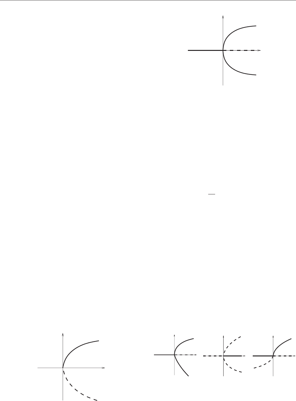
the picture of the solution set in the plane (, x), also
called bifurcation diagram, shows a turning point
with a fold opened to the left or to the right
depending upon the sign of the product @
f (x
0
,
0
)
@
2
x
f (x
0
,
0
); see Figure 1. Notice that here the
bifurcation point (
0
, x
0
) 2 R
2
corresponds to the
appearance of a pair of solutions of [4] ‘‘from
nowhere’’. This is the simplest example of a one-
sided bifurcation in which the bifurcating solutions
exist for either >
0
or <
0
.
A particularly interesting situation arises when the
equation possesses a symmetry. For example, assume
that in [4] the function f is odd with respect to x.This
implies that we always have the solution x = 0, for any
value of the parameter . Assume now that f satisfies
@
x
f ð0;
0
Þ¼0 ½6
and that
@
2
x
f ð0;
0
Þ 6¼ 0;@
3
x
f ð0;
0
Þ 6¼ 0 ½7
Then the point (
0
,0) is a pitc hfork bifurcation
point, this denomination being related with the
bifurcation diagram in the plane (, x); see Figure 2.
Notice that here, the bifurcation point (
0
, x
0
) 2 R
2
corresponds to the bifurcation from the origin of a pair
of solutions exchanged by the symmetry x ! x,in
addition to the persistent ‘ ‘trivial’’ solution x = 0
which is invariant under the above symmetry. Such a
bifurcationisalsoreferredtoasasymmetry-breaking
bifurcation. Similar bifurcation diagrams are found
when the equation [4] has a ‘ ‘known’ ’ branch of
solutions x()for close to
0
. This situation arises
often in applications where usually this branch consists
of trivial solutions x() = 0. Then at a bifurcation
point (
0
, x
0
) a second branch of solutions appears
forming either a one-sided bifurcation, or a two-sided
bifurcation; see Figure 3.
We can now view f as a vector field in the
ordinary differential equation
dx
dt
¼ f ðx;Þ½8
and the study above corresponds to looking for
equilibrium solutions of [8]. The stability of such a
solution is determined by the sign of the derivative
@
x
f (x, )off at this equilibrium, and it is closely
related to the type of the static bifurcation.
In the case of a turning point bifurcation, when
@
2
x
f (x
0
,
0
) 6¼ 0, the sign of @
x
f (x, ) is different for
the two bifurcating solutions. This means that one
solution is attracting (i.e., stable), the other one
being repelling (i.e., unstable); see Figure 1. In the
case of a pitchfork bifurcation as above, the stability
of the trivial solution x = 0 changes when crosses
0
, and the stability of both bifurcating nonzero
solutions is the opposite from the stability of the
origin on the side of the bifurcation. The bifurcation
(µ
0
, x
0
)
µ
x
Figure 1 Turning point bifurcation in the case @
f (x
0
,
0
) > 0
and @
2
x
f (x
0
,
0
) < 0. The solid (dashed) line indicates the branch
of stable (unstable) solutions in the differential equation.
(µ
0
, 0)
µ
x
Figure 2 Supercritical pitchfork bifurcation in the case
@
2
x
f (0,
0
) > 0 and @
3
x
f (0,
0
) < 0.. The solid (dashed) lines
indicate the branch of stable (unstable) solutions in the
differential equation.
(a) (b) (c)
Figure 3 Typical bifurcation diagrams in the case of a branch
of trivial solutions. One-sided bifurcations: (a) supercritical,
(b) subcritical; two-sided bifurcation: (c) transcritical. The solid
(dashed) lines indicate the branch of stable (unstable) solutions
in the differential equation.
276 Bifurcation Theory
is called supercritical if the bifur cating solutions lie
on the side of the bifurcat ion point where the basic
solution x = 0 is unstabl e and subcritical otherwise;
see Figure 2. The situation is the same in the case of
one-sided bifurcations for an equation which has a
‘‘known’’ branch of solutions. In the case of a two-
sided bifurcation, there is an exchange of stability at
the bifurcation point (
0
, x
0
), solutions on the two
branches ha ving opposite stability for >
0
and
<
0
, which changes at (
0
, x
0
). Such a bifurcation
is also referred to as transcritical; see Figure 3.
Notice that the study of fixed points or periodic
points for maps enter in the above frame. Specifi-
cally, the period-doubling process occurring in
successive bifurcations of one-dimensional maps is
a common phenomenon in physics.
The analysis of bifurcations in two dimensions
leads to more complicated scenarios. Consider the
differential equation [8] in which now x 2 R
2
and
f (x, ) 2 R
2
, and assume that f (x
0
,
0
) = 0. The
behavior of solutions near (x
0
,
0
) is determined by
the differential D
x
f (x
0
,
0
)=: L of f with respect to
x, which can be identified with a 2 2 matrix. For
steady solutions, the implicit function theorem
insures the existence of a unique branch of solutions
x() provided L is invertible or, in other words, zero
does not belong to the spectrum of L. Consequently,
the study of bifurcations of steady solutions is
concerned with the case when zero belongs to the
spectrum of L, and can be performed following
the strategy described for one dimension, provided
that the zero eigenvalue of L is simple. For example,
assuming that the second eigenvalue is negative
leads in general to a saddle–node bifurcation, where
an additional dimension is added to the previous
picture of a turning point bifurcation, in which one
of the two bifurcating steady solutions is a stable
node, while the other one is a saddle. If, in addition,
there is a symmet ry S commuting with f, that is,
such that f (Sx, ) = Sf (x, ), and if, for example, x
0
is invariant under S, Sx
0
= x
0
, and the eigenvect or
0
associated to the zero eigenvalue of L is antisym-
metric, L
0
=
0
, then there is again a pitchfork
bifurcation. The equation possesses a branch of
symmetric steady solutions the stability of which
changes when crossing the value
0
of the para-
meter, node on one side and saddle on the other,
and a pair of solutions is created in a one-sided
bifurcation which are exchanged by the symmetry S
and have stability opposite to the one of the
symmetric solution, just as in the one-dimensional
pitchfork bifurcation above.
A new type of bifurcation that arises for vector
fields in two dimensions is the so-called Hopf
bifurcation. This bifurcat ion was first understood
by Poincare´, and then proved in two dimensions by
Andronov (1937) using a Poincare´ map, and later in
n dimensi ons by Hopf (1948) by means of a
Liapunov–Schmidt-type method . For the differential
equation, the absence of the zero eigenvalue in the
spectrum of L is not enough to ensure that the
vector field f ( ,
0
) is structurally stable in a
neighborhood of x
0
. This only holds when the
spectrum of L does not contain purely imaginary
eigenvalues, as asserted by the Hartman–Grobman
theorem. We are then left with the case when L has
a pair of purely imaginary eigenvalues i!, ! 2 R
.
Static bifurcation theory gives that the system has a
unique branch of equilibria (x(), ) for close to
0
, and typically their stability changes as crosses
0
. For the differential equation a Hopf bifurcation
occurs in which a branch of periodic orbits
bifurcates on one side of
0
, and their stability is
opposite to that of the steady solution on this side;
see Figure 4. A convenient way to study this
bifurcation is through ‘‘normal form theory ,’’
which is briefly described below.
Local Bifurcation Theory
There are two aspects of bifurcation theory, local
and global theory. As this designation suggests, local
theory is concerned with (local) properties of the set
of solutions in a neighborhood of a ‘‘known’’
solution, while global theory investigates solutions
in the entire space.
An important class of tools in local bifurcation
theory consists of reduction methods, among which
the Liapunov–Schmidt reduction and the center
manifold reduction are often used to investigate
static and dynamic bifurcations, respectively. The
basic idea is to replace the bifur cation problem by
an equivalent problem in lower dimensions, for
example, a one- or a two-dimensional problem as
the ones above.
Consider again the equation [1] in which F : X
M!Y is sufficiently regular, and X, Y, and M are
Banach spaces. Assume, without loss of generality,
µ
Figure 4 Supercritical Hopf bifurcation.
Bifurcation Theory 277

that F(0, 0) = 0, or, in other words, that one solution
is known. The equation can be then writt en as
LX þ GðX;Þ¼0
in which L = D
X
F(0, 0) represents the differential of
F with respect to X at (0, 0), and is assumed to have
a closed range. The imp licit function theorem shows
absence of bifurcation if L has a bounded inverse, so
that bifurcations are related to the existence of a
nontrivial kernel of L. The Liapunov–Schmidt
reduction then goes as follows.
Let N(L)andR(L) denote the kernel and the range of
L, respectively, and consider continuous projections
P : X!N(L)andQ : Y!R(L). Then there exists a
bounded linear operator B : R(L) !(id P)X,theright
inverse of L, satisfying LB = id on R(L)andBL = id P
on X.ForX 2Xone may write
X ¼ X
0
þ X
1
; X
0
¼ PX; X
1
¼ðid PÞX
and then by projecting with id Q and Q the
equation becomes
ðid QÞGðX
0
þ X
1
;Þ¼0
X
1
þ BQGðX
0
þ X
1
;Þ¼0
The implicit function theorem allows to solve the
second equation for X
1
= (X
0
, ) in a neighborhood
of the origin. Substitution into the first equation leads
to the equation in (id Q) Y for X
0
in PX,
ðid QÞGðX
0
þ ðX
0
;Þ;Þ¼0
also called bifurcation equation. This equation
completely describes the set of solutions to [1] in a
neighborhood of (0, 0), and this problem is then
posed in a space of dimension much smaller than the
dimension of X.
The basic principle of the Liapunov–Schmidt method
has been discovered and used independently by different
authors. E Schmidt (1908) used this method for integral
equations, while Liapunov used it to study the stability
of the zero solution of nonlinear partial differential
equations when the linear part has zero eigenvalues
(1947), and later in 1960 for the bifurcation problem
studied by Poincare´ (1885). In working in a Banach
space of t-periodic functions, the Liapunov–Schmidt
method may be used to solve the Hopf bifurcation
problem, as did Hopf himself in 1948.
The analog of this reduction procedure for the
differential equation [3] is the center manifold
reduction. Assuming that F(0, 0) = 0, we obtain the
differential equation
dX
dt
¼ LX þ GðX;Þ
Since dynamic bifurcations are related to the existence
of purely imaginary spectral values of L, the kernel of L
alone is not enough to describe this situation. One has to
consider the spectral space Y
c
of L associated to the
purely imaginary spectrum of L. A spectral gap is
needed between this part of the spectrum and the rest
(always true in finite dimensions), so that the spectral
projection P onto Y
c
is well defined. One writes
X ¼ X
c
þ X
h
; X
c
¼ PX; X
h
¼ðid PÞX
and obtains the decomposed syst em
dX
c
dt
¼LX
c
þ PGðX
c
þ X
h
;Þ
dX
h
dt
¼LX
h
þðid PÞGðX
c
þ X
h
;Þ
The reduction procedure works provided the non-
homogeneous linear equation
dX
h
dt
¼LX
h
þ f ðtÞ
possesses a unique solution in suitably chosen
function spaces with weak exponential growth,
such that one can then solve the second equation
for X
h
=(X
c
) in a neighborhood of the origin in
these function spaces. This property is always true in
finite dim ensions, but it has to be checked in infinite
dimensions. Different results showing the solvability
of this equation are available in both Banach and
Hilbert spaces, relying upon additional conditions
on the spectrum of L, decaying properties of the
resolvent of L on the imaginary axis, and regularity
properties of the nonlinearity G. The map is then
used to construct a map : PXM!(id P)X,
defined in a neighborhood of the origin, which
parametrizes a local center manifold invariant under
the flow of the equation. The flow on this center
manifold is governed by the reduced equation in Y
c
,
dX
c
dt
¼LX
c
þ PGðX
c
þ ðX
c
;Þ;Þ
which completely describes the bifurcation problem.
The first proofs of this result were given in finite
dimensions by Pliss (1964) and Kelley (1967). Center
manifolds in infinite dimensions have been studied in
different settings determined by assumptions on the
linear part L and the nonlinear part G. One typical
assumption in infinite dimensions is that the spectrum
of L contains only a finite number of purely imaginary
eigenvalues, so that the reduced equation above is a
differential equation in a finite-dimensional space.
These reduction methods work for a large class of
problems and the advantage of such an approach is
that one is left with a bifurcation problem in a
lower-dimensional space. The methods involved in
278 Bifurcation Theory

solving this reduced bifurcation problem can be very
different from one problem to another, and often
make use of some additional structure in the problem,
such as a gradient-like structure, Hamiltonian
structure, or the presence of symmetries, which
are preserved by the reduction procedure.
A powerful tool for the analysis of these reduced
differential equations is provided by the normal
form theory, which goes back to works of Poincare´
(1885) and Birkhoff (1927). The idea is to use
coordinate transformations to make the expression
of the vector field as simple as possible. The
transformed vect or field is called normal form.
There is an extensive literature on normal forms
for vector fields in many different contexts, in both
finite- and infinite-dimensional cases. Typically the
classes of normal forms are characterized in terms of
the linear part of the differential equation.
For differential equations of the form
dx
dt
¼Lx þ gð x;Þ½9
in which L is a matrix and g a sufficiently regular
map such that g(0, 0) = 0, D
x
g(0, 0) = 0, as encoun-
tered in bifurcation theory, one possible character-
ization of normal forms makes use of the adjoint
matrix L
. Fixing any order k 2, there exist
polynomials and N of degree k in x with
coefficients which are regular functions of ,
and (0, 0) = N(0, 0) = 0, D
x
(0, 0) = D
x
N(0, 0) = 0,
such that by the change of variables
x ¼ y þ ðy;Þ
the equation [9] is transformed into the normal form
dy
dt
¼Ly þ Nðy ;Þþoðkyk
k
Þ½10
in which the polynomial N is characterized through
Nðe
tL
y;Þ¼e
tL
Nðy;Þ
for all y, , and t, or, equivalently,
D
y
Nðy;ÞL
y ¼ L
Nðy;Þ
for all y and . This characterization allows to determine
the classes of possible normal forms for a given matrix L,
andalsoprovidesanefficientwaytocomputethe
normal form for a given vector field g.Asforthe
reduction methods, normal form transformations can be
made to preserve the additional structure of the
problem, such as Hamiltonian structure or symmetries.
As an example, consider a differential equation of
the form [9] with x 2 R
n
and 2 R, which supports a
Hopf bifurcation so that L has simple eigenvalues
i!, !>0, and no other eigenvalues with zero real
part. The center manifold reduction provides a
two-dimensional reduced system with linear part
having the simple eigenvalues i!,forwhichitis
convenient to write the normal form in complex
variables
dA
dt
¼ i!A þ AQ
A
2
;
þ o
A
2kþ2
for A(t) 2 C, where Q is a complex polynomial of
degree k in jAj
2
with Q(0, 0) = 0, or, equivalently, in
polar coordinates A = re
i
,
dr
dt
¼ rQ
r
r
2
;
þ o
r
2kþ2
d
dt
¼ ! þ Q
r
2
;
þ o
r
2kþ1
Q
r
and Q
being the real and imaginary part of Q,
respectively. The radial equation for r truncated at
order 2k þ 1 decouples and admits a pitchfork bifurca-
tion. The bifurcating steady solutions of this equation
then lead first to periodic solutions for the truncated
system, which are then shown to persist for the full
equation by a standard perturbation analysis.
A situation that occurs in a large class of problems
is when the problem possesses a reversibility
symmetry, which often comes from some reflection
invariance in the physical space, that is, when the
vector field F( , ) anticommutes with a symmetry
operator S. One of the simplest examples is the case
of a differential equation [9] when the matrix L has
a double eigenvalue in 0, no other eigenvalues with
zero real part, and a one-dimensional kernel which
is invariant by S. In this case, the center manifold
reduction provides a two-dimensional reduced rever-
sible system, which can be put in the normal form
da
dt
¼b
db
dt
¼ a
2
þ oððjajþjbjÞ
3
Þ
which anticomm utes with the symmetry
(a, b) 7!(a, b). The above syst em undergoes a
reversible Takens – Bogdanov bifurcation and has
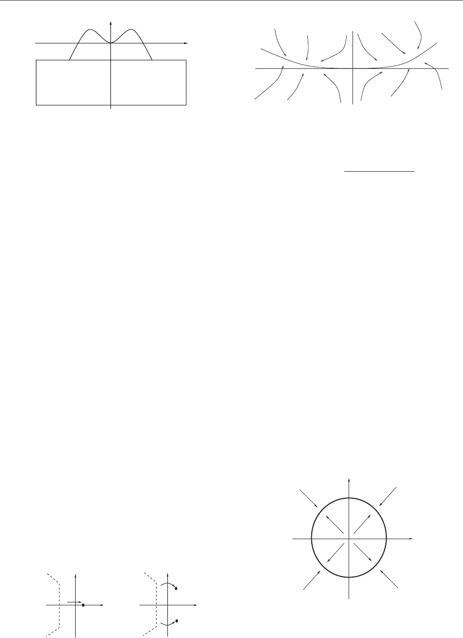
for >0 a phase portrait as in Figure 5. There are
two equilibria, one a saddle, the other a center, and
a family of periodic orbits with the zero-amplitude
limit at the center equilibrium, and the infinite-
period limit a homoclinic orbit, originating at the
saddle point. In concrete problems the bounded
orbits of such a reduced system determine the shape
of physically interesting solutions of the full system
of equations, such as, for example, in water-wave
theory where to homoclinic and periodic orbits
correspond solitary and periodic waves, respe ctively.
Bifurcation Theory 279
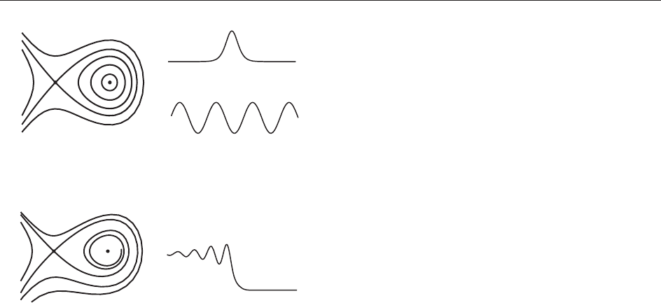
Notice that in the absence of the reversibility
symmetry, the same type of bifurcation may lead to
a completely different phase portrait for the reduced
system as, for example, the one in Figure 6 in which
the homoclini c and the periodic orbits disappear.
This situation often occurs in the presence of a small
dissipation in nearly reversible systems.
Global Bifurcation Theory
Most of the existing results in global bifurcation
theory concern the static problem [1]. The analysis
of global sets of solutions often relies upon
topological methods, degree theory, but also varia-
tional methods, or analytic function theory. Signifi-
cant progress in understanding global branches of
solutions has been made in the 1970s, in particular,
for nonlinear eige nvalue problems and the Hopf
bifurcation problem (see, e.g., works by Rabinowitz,
Crandall, Dancer, and Alexand er, Yorke, Ize,
respectively).
A now-classi cal result in the topological theory of
global bifurcations is the following theorem by
Rabinowitz (1970), which give s a characterization
of global sets of solutions for eigenvalue problems of
the form
X ¼ FðX;Þ¼LX þ HðX;Þ
H(X, ) ¼o(kXk), posed for (X, ) 2XR, X being
a Banach space. In contrast to local theory where
the function F is usually k-times differentiable (with
a suitable k), in the global theory a typical
assumption is that F : XR !X is compact. The
equation above possesses a ‘‘trivial’’ branch of
solutions (0, ) for any . The bifurcation result
asserts that if for some real parameter value
0
zero
is an eigenvalue of odd multiplicity of the operator
id
0
L, then the set S of nontrivial solutions (X, )
possesses a maximal subcontinuum which contains
(0,
0
) and meets either infinity in XR or another
trivial solution (0,
1
),
1
6¼
0
. In particular, (
0
,0)
is a bifurcation point. A local version of this result is
often referred to as Krasnoselski’s theorem.
Different versions and extensions of these theo-
rems can be found in the literature, as, for example,
in the case of a simple eigenvalue, or if the field F is
real-analytic when the set of solutions is path-
connected. More recent works address the question
of lack of compactness, and a number of results are
now available for problems with additional struc-
ture (gradient-like or Hamiltonian structure), but
also for concrete problems, such as the water-wave
problem.
See also: Bifurcations in Fluid Dynamics; Bifurcations of
Periodic Orbits; Central Manifolds, Normal Forms;
Dynamical Systems in Mathematical Physics: An
Illustration from Water Waves; Ginzburg–Landau
Equation; Integrable Systems: Overview; Leray–
Schauder Theory and Mapping Degree; Singularity and
Bifurcation Theory; Stability Theory and KAM; Symmetry
and Symmetry Breaking in Dynamical Systems.
Further Reading
Arnold VI (1988) Geometrical Methods in the Theory of
Ordinary Differential Equations. Grundlehren der Mathema-
tischen Wissenschaften, vol. 250. New York: Springer.
Buffoni B and Toland J (2003) Analytic Theory of Global
Bifurcation. Princeton: Princeton University Press.
Chossat P and Lauterbach R (2000) Methods in Equivariant
Bifurcations and Dynamical Systems. Advanced Series in
Nonlinear Dynamics, vol. 15. River Edge, NJ: World
Scientific.
Chow S-N and Hale JK (1982) Methods of Bifurcation Theory.
Grundlehren der Mathematischen Wissenschaften, vol. 251.
New York: Springer.
Golubitsky M and Schaeffer DG (1985) Singularities and Groups
in Bifurcation Theory, Vol. I. Applied Mathematical Sciences,
vol. 51. New York: Springer.
Golubitsky M, Stewart I, and Schaeffer DG (1988) Singularities
and Groups in Bifurcation Theory, Vol. II. Applied Mathema-
tical Sciences, vol. 69. New York: Springer.
Guckenheimer J and Holmes P (1990) Nonlinear Oscillations,
Dynamical Systems, and Bifurcations of Vector Fields. Applied
Mathematical Sciences, vol. 42. New York: Springer.
Iooss G and Adelmeyer M (1998) Topics in Bifurcation Theory
and Applications, Advances Series in Nonlinear Dynamics,
2nd edn., vol. 3, Singapore: World Scientific.
Iooss G, Helleman RHG, and Stora R (eds.) (1983) Chaotic
behavior of deterministic systems. Session XXXVI of the
Summer School in Theoretical Physics held at Les Houches
June 29–July 31, 1981. Amsterdam: North-Holland.
Figure 5 Phase portrait of the reduced system in a reversible
Takens–Bogdanov bifurcation (left) and sketch of the a-component
of solutions corresponding to homoclinic and periodic orbits (right).
Figure 6 Phase portrait of the reduced system in absence of
reversibility (left) and sketch of the a-component of the solution
corresponding to the bounded orbit (right).
280 Bifurcation Theory
Ize J and Vignoli A (2003) Equivariant Degree Theory. de
Gruyter Series in Nonlinear Analysis and Applications, vol. 8.
Berlin: de Gruyter and Co.
Kielho¨ fer H (2004) Bifurcation Theory. An Introduction with
Applications to PDEs, Applied Mathematical Sciences,
vol. 156. New York: Springer.
Kuznetsov YA (2004) Elements of Applied Bifurcation Theory,
3rd edn. Applied Mathematical Sciences, vol. 112. New York:
Springer.
Ruelle D (1989) Elements of Differentiable Dynamics and
Bifurcation Theory. Boston MA: Academic Press.
Vanderbauwhede A (1989) Centre Manifolds, Normal Forms and
Elementary Bifurcations. Dynamics Reported, Dynam. Report.
Ser. Dynam. Systems Appl.,vol.2,pp.89–169.Chichester:Wiley.
Vanderbauwhede A and Iooss G (1992) Center Manifold Theory
in Infinite Dimensions. Dynamics Reported: Expositions in
Dynamical Systems, vol. 1, pp. 125–163. Berlin: Springer.
Bifurcations in Fluid Dynamics
G Schneider, Universita
¨
t Karlsruhe, Karlsruhe,
Germany
ª 2006 Elsevier Ltd. All rights reserved.
Introduction
Almost all classical hydrodynamical stability problems
are experiments or gedankenexperiment which have
been designed to understand and to extract special
phenomena in more complicated situations. Examples
are the Taylor–Couette problem, Be´nard’s problem,
Poiseuille flow, or Kolmogorov flow.
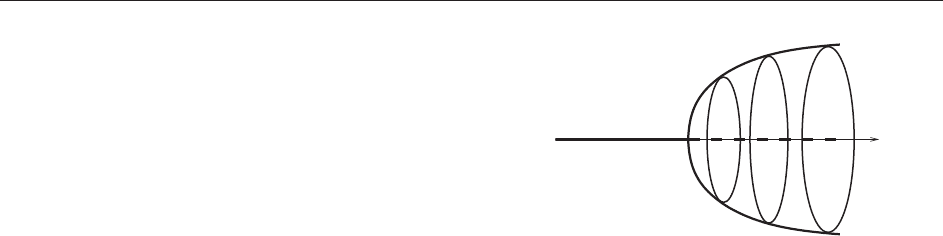
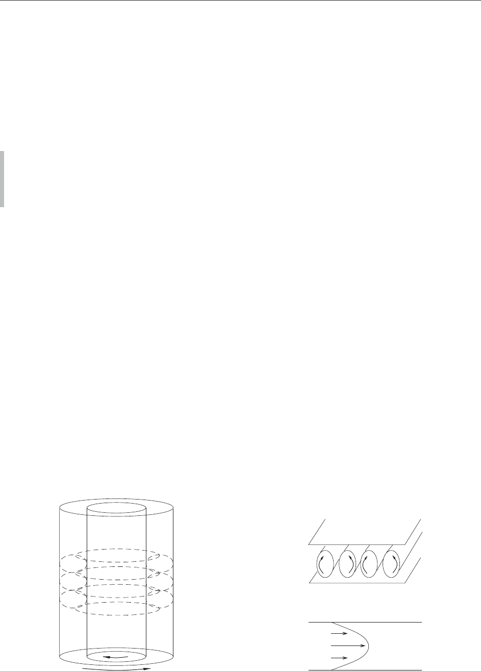
The Taylor–Couette problem consists in finding the
flow of a viscous incompressible fluid contained in
between two coaxial co- or counterrotating cylinders,
cf. Figure 1. If the rotational velocity of the inner
cylinder is below a certain threshold, the trivial
solution, called the Couette flow, is asymptotically
stable. At the threshold, this spatially homogenous
solution becomes unstable and bifurcates via a pitch-
fork bifurcation or a Hopf bifurcation into different
spatially periodic patterns, that is, depending on the
rotational velocity of the outer cylinder the basic
patterns are stationary (called the Taylor vortices) or
time-periodic. If the rotational velocity of the inner
cylinder is increased further, more complicated pat-
terns occur. The bifurcation scenario is well under-
stood from experiments and analytic investigations.
Be´nard’s problem consists in finding the flow of a
viscous incompressible fluid contained in between two
plates, where the lower plate is heated and the upper
plate is kept at a constant temperature, cf. Figure 2.If
the temperature difference between the two plates is
below a certain threshold, the transport of energy from
below to above is made by pure conduction. At this
threshold, this spatially homogenous solution becomes
unstable, convection sets in, and spatially periodic
patterns as rolls or hexagons occur. Convection
problems play a big role in geophysical applications,
that is, in spherical domains, as the earth. The paradigm
for an anisotropic pattern-forming system is electro-
convection in nematic crystals.
Poiseuille flow consists in finding the flow of a
viscous incompressible fluid flowing through a pipe
driven by some press ure gradient, cf. Figure 3.In
noncircular pipes, the trivial laminar flow becomes
unstable at a critical pressure gradient. Experimen-
tally, a direct transition to turbulent flow with large
amplitudes is observed, according to the fact that in
general at the instability point of the trivial solution
a subcritical bifurcation occurs.
Figure 1 The Taylor–Couette problem with the Taylor vortices.
Figure 2 Be
´
nard’s problem with rolls.
Figure 3 Poiseuille flow with the trivial solution.
Bifurcations in Fluid Dynamics 281
Kolmogorov flow consists in finding the flow of a
viscous incompressible fluid under the action of an
external force parallel to the flow direction x and
varying periodically in the perpendicular y-direction.
This gedankenexperiment has been designed by
Kolmogorov in 1958 as a simplified model for the
Poiseuille flow problem in order to study the nature
of turbulence. The trivial solution which is called
Kolmogorov flow can become unstable via a long-
wave instability along the flow direction.
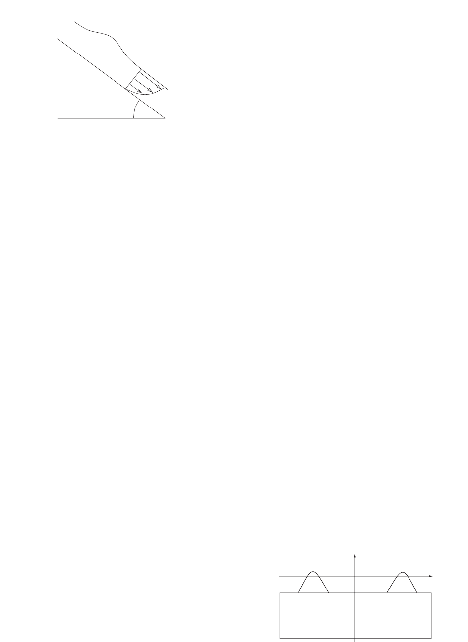
The inclined-plane problem consists in finding the
flow of a viscous liquid running down an inclined
plane, cf. Figure 4. The trivial solution, the so-called
Nusselt solution, becomes sideband-unstable if the
inclination angle is increased. Then the dynamics is
dominated by traveling pulse trains, although the
individual pulses are unstable due to the long-wave
instability of the flat surface. Time series taken from
the motion of the individual pulses indicates the
occurrence of chaos directly at the onset of instability.
There are other famous hydrodynamical stability
problems, with arbitrarily complicated bifurcation
scenarios.
Spectral Analysis of the Trivial Solution
All classical hydrodynamical stability problems are
described by the Navier–Stokes equations
@
t
U ¼
1
U rp ðU rÞU þ f
0 ¼rU
½1
where U = U(x, t) 2 R
d
with d = 2, 3 is the velocity
field, p = p(x, t) 2 R thepressurefield,f some external
forcing, and the dynamic viscosity. These equations
are completed with boundary conditions. In case of
Be´nard’s problem, the Navier–Stokes equations are
coupled to a nonlinear heat equation.
By projecting U onto the space of divergence-free
vector fields and by taking the trivial solution as
new origin all problems from the previous section
can be written as evolutionary system
@
t
U ¼ U þ NðU Þ
where U = 0 corresponds to the trivial solution, where
is a linear and N(U) = O(U
2
)forU !0 a nonlinear
operator. Most of the examples from the previous
section are semilinear, that is, from a functional
analytic point of view, the nonlinear operator N can
be controlled in terms of the linear operator .
Since the form of the bifurcating pattern is only
slightly influenced by far away boundaries, that is, for
instance, the upper and lower end of the rotating
cylinders in the Taylor–Couette problem, the problems
are considered from a theoretical point of view in
unbounded domains, =R
d
,with R
m
the
bounded cross section that is, for instance, that the
Taylor–Couette problem is considered with two cylin-
ders of infinite length. Then the eigenfunctions of the
linear operator are given by Fourier modes, that is,
ðe
ikx
’
k;n
ðzÞÞ ¼
n
ðkÞe
ikx
’
k;n
ðzÞ
with x 2 R
d
, k 2 R
d
, k x =
P
d
j = 1
k
j
x
j
, z 2 , n 2 N.
If an external control parameter is changed, inde-
pendent of the underlying physical problem, the
trivial solution becomes unstable, then the surface
k 7!Re
1
(k) intersects the plane {Re
1
(k) = 0}.
Generically, this happens first at a nonzero wave
vector k
c
6¼ 0 (cf. Figure 5).
Examples for such an instability are the Taylor–
Couette problem, Be´nard’s problem, or Poiseuille
flow. Very often, due to some conserved quantity in
the problem we have Re
1
(0) = 0 for all values of
the bifurcation parameter. Then, a so-called side-
band instability can occur, cf. Figure 6.
Examples for such an instability are the Kolmo-
gorov flow problem or the inclined plane problem.
According to some symmetries in the problem, for
instance, reflection along the cylinders in the
Taylor–Couette problem or rotational symmetry in
Be´nard’s problem, the curves in Figure 5 are double
or rotational symmetric.
In case of being spherical symmetric, we have
ðf
l
ðrÞ’
l; n
ðzÞÞ ¼
l
f
l
ðrÞ’
l; n
ðzÞ
φ
Figure 4 The inclined-plane problem. The trivial Nusselt
solution possesses a flat top surface and a parabolic flow profile.
k
Rest of spectrum
Figure 5 Real part of the spectrum in case of an instability at a
wave number k
c
6¼ 0. Definition of the small bifurcation parameter ".
282 Bifurcations in Fluid Dynamics
with r 0, z 2 S
d
, ’
l, n
for l 2 N
0
and m = l,
l 1, ..., l þ 1, l being a spherical harmonic, that
is, if
l
0
is the eigenvalue having first positive real
part, then by symmetry, simultaneously 2l
0
þ 1
eigenvalues cross the imaginary axis.
Reduction of the Dimension
In order to understand the occurrence of the spatially
periodic Taylor vortices in the Taylor–Couette pro-
blem and of the roll solutions and hexagons in
Be´nard’s problem, the problems are considered with
periodic boundary conditions along the unbounded
directions. Then the instability of the trivial solution
occurs when at least one eigenvalue crosses the
imaginary axis. Generically, this happens by a simple
real eigenvalue or a pair of complex-conjugate
eigenvalues crossing the imaginary axis (Figure 7).
Center manifold theory and the Lyapunov–Schmidt
reduction allow to reduce the aprioriinfinite-dimen-
sional bifurcation problem to a finite-dimensional one.
In case of a real eigenvalue
1
crossing the imaginary
axis, the solution u can be written as a sum of the
weakly unstable mode and the stable modes, that is,
u = c
1
’
1
þ u
r
,(c
1
2 R), where u
r
lives in the closure of
the span of the stable eigenfunctions {’
2
, ’
3
, ...}. For
the linearized system all solutions are attracted by the
one-dimensional set E
c
= {u ju
r
= 0}, in which all
solutions diverge to infinity.
For the nonlinear system and small bifurcation
parameter this attracting structure survives, no
longer as a linear space, but as a manifold
M
c
¼fu ¼ c
1
’
1
þ hðc
1
Þj
hðc
1
Þ2spanf’
2
;’
3
; ...gg
the so-called center manifold which is tangential to E
c
,
that is, kh(c
1
)kCkc
1
k
2
(Figure 8). The dynamics on
M
c
is no longer trivial due to the nonlinear terms.
Due to the fact that real problems are considered
Re
1
(k
c
) = 0 implies Re
1
(k
c
) = 0, that is, in case
of 2=k
c
-periodic boundary conditions always two
eigenvalues cross the imaginary axis simultaneously.
For Be´nards’s problem in a strip or for the Taylor–
Couette problem in case of a bifurcation of fixed
points, the reduced system on the center manifold is
derived with the ansatz
U ¼ "Að"
2
tÞe
ik
c
x
þ c:c: þOð"
2
Þ
where 0 <" 1 is the small bifurcation parameter,
cf. Figure 5. Then due to e
ik
c
x
e
ik
c
x
e
ik
c
x
= e
ik
c
x
the
complex-valued amplitude A satisfies the so-called
Landau equation
@
T
A ¼ A AjAj
2
þOð"
2
Þ
where the Landau coefficient 2 R is obtained by
classical perturbation analysis (Figure 9). The
reduced system is symmetric under the S
1
-symmetry
k
Rest of spectrum
Figure 6 Real part of the spectrum in case of a sideband
instability. Definition of the small bifurcation parameter ".
Rest of
spectrum
Rest of
spectrum
Figure 7 Generically, a simple real eigenvalue or a pair of
complex-conjugate eigenvalues cross the imaginary axis.
E
c
M
c
E
s
Figure 8 The center manifold is invariant under the flow, is
tangential to the central subspace E
c
, and attracts nearby
solutions with some exponential rate.
Im
Re
Figure 9 The dynamics of the Landau equation. Except of the
origin which corresponds to the Couette flow, all solutions
converge towards the circle of fixed points, which corresponds
to the family of Taylor vortices. The translation invariance of the
Taylor–Couette problem is reflected by the rotational symmetry of
the reduced system.
Bifurcations in Fluid Dynamics 283
A 7!Ae
i
with 2 R which corresponds to the
translation invariance of the original systems.
This so-called equivariant bifurcation theory has
been applied succe ssfully to convection problems in
the plane and on the sphere.
The stability of time-periodic flows can be
analyzed with Floquet multipliers. Bifurcations
from a time-periodic solution can lead to quasiper-
iodic motion in time. Ruelle and Takens (1971)
showed that already the next bifurcation leads to
chaotic dynamics. Since this time many classical
hydrodynamical stability problems have been ana-
lyzed with bifurcation theory up to turbulent flows.
It was observed that center manifold theory can
also be applied successfully to elliptic PDE problems
posed in spatially unbounded cylindrical domains.
A famous example is the construction of capillary-
gravity solitary waves for the so-called water-wa ve
problem.
Modulation Equations
The analysis of the last section is of no use in case of
a sideband instability occurring at the wave number
k
c
= 0, as it happens in the inclined-plane problem
or in the Kolmogorov flow problem. Moreover, in
case of an instability at a wave vector k
c
6¼ 0, based
on the above analysis, front solutions cannot be
described. In such situations, the method of modula-
tion equations generalizes the role of the finite-
dimensional amplitude equations from the last
section.
The complex cubic Ginzburg–Landau equation in
normal form is given by
@
T
A ¼ð1 þ iÞ@
2
X
A þ A ð1 þ iÞAjAj
2
where the coefficients , 2 R are real, and we have
X 2 R, T 0, and A(X , T) 2 C. The Ginzburg–
Landau equation is a universal amplitude equation
that describes slowly varying modulations, in space
and time, of the amplitude of bifurcating spatially
periodic solutions in pattern-forming systems close
to the threshold of the first instability. Whenever the
instability drawn in Figure 5 occurs, that is, for the
Taylor–Couette problem and Be´nard’s problem in a
strip, that is, d = 1, it can be derived by a multiple
scaling ansatz
uðx; tÞ"Að"ðx c
g
t Þ;"
2
tÞe
iðk
c
x!
0
tÞ
þ c:c:
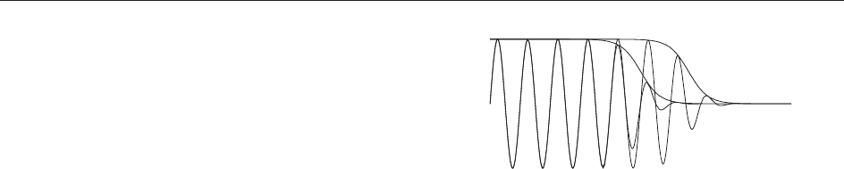
For instance, in case of = = 0, the Ginzburg–
Landau equation possesses front solutions connect-
ing the stable fixed point A = 1 with the unstable
fixed point A = 0. Such solutions correspond in the
Taylor–Couette problem to modulating fronts
connecting the stable Taylor vortices with the
unstable Couette flow, cf. Figure 10 .
The diffusion operator in the Ginzburg–Landau
equation reflects the parabolic shape of Re
1
close
to k = k
c
in Figure 5. In case of the long-wave
instability, as drawn in Figure 6, the second-order
differential operator changes in a fourth-order
differential operator.
For Kolmogorov flow with T = "
4
t and X = "x and
the amplitude scaled with ",weobtainthatinlowest
order A has to satisfy a Cahn–Hilliard equation
@
T
A ¼
ffiffiffi
2
p
@
2
X
A 3@
4
X
A þ @
2
X
ðA
3
Þ
where A(X, T) 2 R and 2 R a constant (cf. Figure 6).
The Kuramoto–Shivashinsky (KS)-perturbed KdV
equation
@
T
A ¼@
3
X
u @
X
ðA
2
Þ=2 "ð@
2
x
þ @
4
x
Þu
with A =A(X,T) 2R, X 2R, T 0, where 0 <"1
is still a small parameter, can be derived for the
inclined problem with T = "
3
t and X = "x and the
amplitude scaled with "
2
.
The theory of modulation equations is nowadays a
well-established mathematical tool which allows us to
construct special solutions, global existence results for
the solutions of pattern-forming systems, or allows to
characterize the attractors in such systems. The
method is based on approximation results, showing
that solutions of the original systems can be approxi-
mated by the modulation equation and attractivity
results showing that every solution of the original
system develops in such a way that it can be described
by the modulation equation.
This method can also be applied to secondary
bifurcations describing instabilities of spatially per-
iodic wave trains. Then the so-called phase-diffusion
equations, conservation laws, Burgers equations,
and again the KS equations occur.
However, this met hod cannot be applied success-
fully in all situations. There are counterexamples
showing that not every formally derived modulation
equation describes the original system in a correct
way. Moreover, very often according to some
symmetries in the original problem no consistent
Figure 10 The front solution of the Ginzburg–Landau equation
modulates the underlying pattern in the original system.
284 Bifurcations in Fluid Dynamics