Francoise J.-P., Naber G.L., Tsun T.S. (editors) Encyclopedia of Mathematical Physics
Подождите немного. Документ загружается.

multiple scaling analysis is possible, that is, that the
modulation equations still depend on ".
Discussion
There is no satisfactory bifurcation analysis for situa-
tions where boundary layers play a role. The most
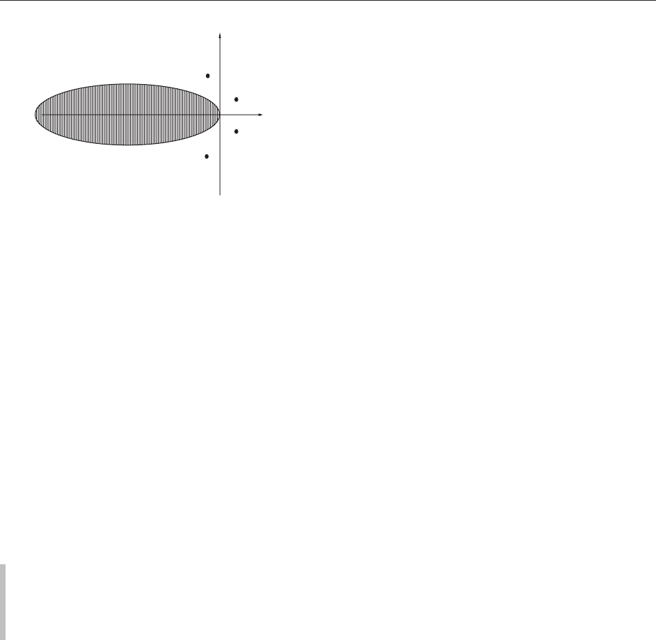
simple problem is the flow around some obstacle. The
difficulties are according to the fact that due to the
unbounded flow region there is always continuo us
spectrum up to the imaginary axis. From the localized
obstacle discrete eigenvalues are created, (cf. Figure 11).
In such a situation, so far there is no mat hematical
bifurcation theory available.
See also: Bifurcation Theory; Dynamical Systems in
Mathematical Physics: An Illustration from Water Waves;
Leray–Schauder Theory and Mapping Degree; Multiscale
Approaches; Newtonian Fluids and Thermohydraulics;
Symmetry and Symmetry Breaking in Dynamical Systems;
Turbulence Theories; Variational Methods in Turbulence.
Further Reading
Chandrasekhar S (1961) Hydrodynamic and Hydromagnetic
Stability. Oxford: Clarendon.
Chang H-C and Demekhin EA (2002) Complex Wave Dynamics
on Thin Films, Studies in Interface Science, vol. 14. Amsterdam:
Elsevier.
Chossat P and Iooss G (1994) The Taylor–Couette Problem,
Applied Mathematical Sciences, vol. 102. Springer.
Chow S-N and Hale J (1982) Methods of Bifurcation Theory,
Grundlehren der Mathematischen Wissenschaften, vol. 251.
Berlin: Springer.
Golubitsky M and Schaeffer DG (1985) Singularities and Groups
in Bifurcation Theory I, Applied Mathematical Sciences,
vol. 51. Berlin: Springer.
Golubitsky M, Stewart I, and Schaeffer DG (1988) Singularities
and Groups in Bifurcation Theory II, Applied Mathematical
Sciences, vol. 69. Berlin: Springer.
Haken H (1987) Advanced Synergetics. Berlin: Springer.
Henry D (1981) Geometric Theory of Semilinear Parabolic Equa-
tions, Lecture Notes in Mathematics, vol. 840. Berlin: Springer.
Mielke A (2002) The Ginzburg–Landau equation in its role as a
modulation equation. In: Fiedler B (ed.) Handbook of Dyna-
mical Systems II, pp. 759–834. Amsterdam: North-Holland.
Ruelle D and Takens F (1971) On the nature of turbulence.
Communications in Mathematical Physics 20: 167–192.
Temam R (1988) Infinite-Dimensional Systems in Mechanics and
Physics. Berlin: Springer.
Bifurcations of Periodic Orbits
J-P Franc¸ oise, Universite
´
P.-M. Curie, Paris VI, Paris,
France
ª 2006 Elsevier Ltd. All rights reserved.
Introduction
Bifurcation theory of periodic orbits relates to
modeling of quite diverse subje cts. It appeared
classically in the field of celestial mechanics with
the contributions of H Poincare´. Van der Pol (1926,
1927, 1928, 1931) observed the frequency-locking
phenomenon in electrical circuits. More recently,
Malkin’s theory (Malkin 1952, 1956, Roseau 1966)
was used to justify synchronization of weakly
coupled oscillators modeling the electrical activity
of the cells of the sinusal node in the heart. This
article provides the essential mathematical back-
ground necessary for existence of frequency locking.
Applications can be found, for instance, in Weakly
Coupled Oscillators.
The Asymptotic Phase of a Stable
Periodic Orbit
Let be a periodic orbit of a vector field and let
S() denote the stable manifold of (resp. U()
denotes the unstable manifold of ). The following
theorem can be found, for instance, in Hartman
(1964).
Theorem There exist and K such that Re(
j
) < ,
j = 1, ..., kandRe(
j
) >, j = k þ 1, ..., and for all
x 2 S(), there is an asymptotic phase t
0
such that for
all t 0
j
t
ðxÞðt t
0
Þj< K e
ðt=TÞ
Similarly, for any x 2 U(), there is a t
0
such that t 0,
j
t
ðxÞðt t
0
Þj< K e
ðt=TÞ
If the periodic orbit is stable, the local stable
manifold coincides with an open neighborhood of .
In such a case, there is a foliation of this open set
Re
Im
Continuous spectrum
Discrete eigenvalues
Figure 11 Spectrum for the flow around an obstacle.
Bifurcations of Periodic Orbits 285

whose leaves are the points with a given asympto-
tic phase. The asymptotic phase can be considered
as a coordinate function defined on the
neighborhood S().
If we consider now the particular case of a plane
system, this function can be completed with the
square of the distance function to the orbit into a
coordinate system called the ‘‘amplitude–phase’’
system and denoted as (, ).
Frequency Locking and Phase Locking
The term ‘‘oscillator’’ has two meanings. A con-
servative ‘‘oscillator’’ is a plane vecto r field which
displays an open set of periodic orbits. It is said to
be isochronous if all orbits have same period. A
dissipative ‘‘oscillator’’ is a planar vector field which
displays an attractive limit cycle (attractive periodic
orbit).
We consider N dissipative oscillators:
dx
i
dt
¼ f ðx
i
; y
i
Þ
dy
i
dt
¼ gðx
i
; y
i
Þ
½1
where i = 1, ..., m.
The dynamical system obtained by considering the
space of all the variables ( x
i
, y
i
), i = 1, ..., m, dis-
plays an invar iant torus full of periodic orbits that
we denote by T
m
(0).
Assume now that the N oscillators are weakly
coupled:
dx
i
dt
¼ f ðx
i
; y
i
ÞþF
i
ðx; y;Þ
dy
i
dt
¼ gðx
i
; y
i
ÞþG
i
ðx; y;Þ
½2
where can be considered as small as we wish.
Definition The system [2] has a frequency locking
if it displays a family of stable periodic orbits
for
all values of small enough which tends to (in the
sense of Hausdorff’s topology) a periodic orbit of [1]
contained in the periodic torus T
m
(0).
Assume now that [2] has a frequency locking
associated with the periodic orbit (t). Consider the
projections
i
(t)of(t) on the coordinates plane
(x
i
, y
i
), i = 1, ..., m. Assume that is small enough
so that the projection belongs to the open set S
i
on
which are defined the ‘‘amplitude–phase’’ coordi-
nates of the system [1]. We can write the system [2],
restricted to the open set S =
m
i=1
S
i
,as
d
i
dt
¼ f
i
ð; ; Þ
d
i
dt
¼ F
i
ð; ; Þ; i ¼ 1; ...; m
½3
Definition The system [2] has a phase locking if
the system induced by [3] on (t)
d
i
dt
¼ F
i
ð0;;Þ½4
has an attractive singular point.
As the attractive singular points are structurally
stable, this is enough to assume that the system
d
i
dt
¼ F
i
ð0;;0Þ½5
displays an attractive singular point.
Periodic Orbits of Linear Systems
Consider the linear system
dx
dt
¼ PðtÞx þ qðtÞ½6
where P is a continuous T-periodic matrix function
and q is a vector T-periodic continuous function,
x = (x
1
, ..., x
n
). Consider also the two associated
homogeneous equations:
dx
dt
¼ PðtÞx ½7a
dx
dt
¼P
ðtÞx ½7b
where P
denotes the transposed of P.
The set of T-periodic solutions of [7b] is a vector
space. m denotes its dimension. Let U
j
(t), j = 1, ..., m,
be a basis of this vector space. This basis is completed
by adding n m solutions U
j
(t), j = m þ 1, ..., n,to
obtain a basis of R
n
.LetU(t ) be the matrix whose
columns are these vectors; denote U
ij
(t) the elements of
this matrix.
With the change of variable x = U
(0)
1
y, system
[6] gets transformed into
dy
dt
¼ QðtÞy þ rðtÞ½8
with Q(t) = U
(0)P(t) U
(0)
1
and r(t ) = U
(0)q(t).
Matrix V(t) = U
1
(0)U(t) is such that
dV
dt
þ Q
ðtÞV ¼ 0; Vð0Þ¼I
286 Bifurcations of Periodic Orbits

and the k first column vectors V(t), denoted as
V
j
(t), j = 1, ..., m, are T-periodic.
Let X(t) be the fundamental solution defined by
dX
dt
¼ Qð tÞX; Xð0Þ¼I
then,
X
1
ðtÞ¼V
ðtÞ
The solution of [8] can be written as
yðtÞ¼Xð tÞyð0ÞþXðtÞ
Z
t
0
X
1
ðuÞrðuÞdu ½9
This yields that T-periodic solutions of [8] have
initial data y(0) given by
ðV
ðTÞIÞyð0Þ¼
Z
T
0
V
ðsÞrðsÞds ½10
Conversely, given a solution y(0) of [10],
T-periodicity of P and q and uniqueness of solutions
of a differential equation imply that y(0) represents the
initial data of a T-periodic solution of [8]. Hence, the
T-periodic solutions of [8] are in one-to-one corre-
spondence with the affine space defined by the
solutions of [10].Them first rows of V
(T) I are
zero and its rank is exactly n m. In the following,
assume that the determinant formed by the (n m)
last rows and last columns of (V
(T) I) is not zero.
A necessary and sufficient condition so that [8]
displays a T-periodic solution is
Z
T
0
X
n
j¼1
V
jk
ðuÞr
j
ðuÞdu ¼ 0; k ¼ 1; ...; m ½11a
X
n
j¼mþ1
ðV
jk
ðTÞ
jk
Þy
j
ð0Þ
¼
X
n
j¼1
Z
T
0
V
jk
ðsÞr
j
ðsÞds; m þ 1 s n ½11b
This yields the Fredholm alternative, if the m
conditions,
X
n
j¼1
Z
T
0
U
jk
ðsÞq
j
ðsÞds ¼ 0; k ¼ 1; ...; m ½12
are satisfied, t hen [6] displays a f amily x
(t)of
T-periodic solutions depending o f m parameters
(
1
, ...,
m
):
x
ðtÞ¼
1
1
ðtÞþþ
m
m
ðtÞþ
xðtÞ½13
where
x(t) is a particular T-periodic solution and
j
(t) denote T-periodic independent solutions of
[7a]. To be more specific, one can choose
x(t)to
be the unique solution of [6] such that
y(0)
k
= 0, k = m þ 1, ..., n, and
j
(t) solutions of
[7a], such that y(0)
k
=
jk
. With these notations,
x
(t) is such that
yð0Þ
k
¼
k
; k ¼ 1; ...; m
and its other initial conditions y(0)
k
=
k
, k = m þ
1, ..., n, are fixed:
k
¼
0
k
Malkin’s Theorem for Quasilinear
Systems
Consider now nonlinear systems with the
perturbation:
dx
dt
¼ PðtÞx þ qðtÞþf ðx; t;Þ½14
where f is C
1
and T-periodic in t.
Assume that the solutions y(t, y (0), )of[14] exist
for all values of t,0 t T. The solutions define a
differential function of their initial data y(0). This is,
for instance, true for perturbations of linear systems
if is small enough.
Assume that q satisfies la condition [12] and that
there is a solution
0
1
; ...;
0
m
to the equations
k
ðÞ¼
X
n
j¼1
Z
T
0
U
jk
ðuÞf
j
ðx
ðuÞ; u; 0Þdu ¼ 0;
k ¼ 1; ...; m ½15a
so that
@
k
ðÞ
@
j
j
¼
0
; k ¼ 1; ...m; j ¼ 1; ...; m ½15b
is invertible.
Proceed as in previous section with the coordinate
change x = U
(0)
1
y. Equation [14] gets trans-
formed into
dy
dt
¼ QðtÞy þ rðtÞþFðy; t;Þ½16
with F = U
(0)f (U
(0)
1
y, t, ).
Solutions of [16] are uniquely determined by their
initial data. We can understand the parameters (, )
as coordinates on the space of solutions. With this
viewpoint, for instance, the set of T-periodic
solutions of [6] is an affine space of dimension m
Bifurcations of Periodic Orbits 287

given by the equations =
0
and is parametrized by
the coordinates . In this space, we pick up a point
(which corresponds to a particular T-periodic solu-
tion of [6]): ( =
0
). T-periodic solutions of [16] are
in one-to-one correspondence with the solutions of
C
k
ð; ; Þ¼
X
n
j¼1
Z
T
0
V
jk
ðsÞF
j
ðyðs;;;Þ; s;Þds ¼ 0;
k ¼ 1; ...; m ½17a
C
k
ð; ; Þ¼
X
j¼mþ1;...;n
ðV
jk
ðTÞIÞ
j
X
n
j¼1
Z
T
0
V
jk
ðsÞr
j
ðsÞds
X
n
j¼1
Z
T
0
V
jk
ðsÞF
j
ðyðs;;;Þ; s;Þds ¼0;
k ¼ m þ 1; ...; n ½17b
where
k
, k = 1, ..., m and
k
= y
k
(0), k = m þ
1, ..., n param etrize the solutions y(t, , , )of
[14] in this way:
yð0Þ¼U
ð0Þxð0Þ; xð0Þ¼
X
m
j¼1
j
j
ð0Þþ
xð0Þ½18
Consider the determinant of the Jacobian matrix
of the mapping
ð; Þ7!Cð; ; Þ½19
for =
0
,
k
=
0
k
, k = m þ 1, ..., n , = 0. This is
equal to the product of and the determinant of
@
k
ðÞ
@
j
j
¼
0
½20
which is nonzero.
The implicit-function theore m shows that the
differential equation [14] (and thus [16] as well)
has, for small enough, a unique T-periodic solution
which tends to x
0
when tends to 0.
Generalization of Malkin’s Theorem
Finally, we consider the most general situation of
the perturbation of a general system (not necessarily
linear):
dx
dt
¼ f ðx; tÞþgðx; t;Þ½21
where we assume that
dx
dt
¼ f ðx; tÞ½22
displays an m-parameter family x
(t)ofT-periodic
orbits.
Assume that the solutions y(t, y(0), ) exist for all
0 t T and define a differentiable mapping of the
initial data y(0). This is, for instance, the case if we
assume that the nonperturbed equation defines a
flow and if is small enough.
Assume also that the different solutions x
(t) are
independent in the sense that the mapping
7!x
ðtÞ
is an immersion for any t. In other words, the m
vectors dx
(t) =d
j
are independent.
We linearize the solution along the family of
periodic orbits:
x ¼ x
ðtÞþ ½23
Equation [21] gets transformed into
d
dt
¼Df
x
ðx
ðtÞ;tÞ þgðx
ðtÞ;t; 0ÞþFð;t;Þ½24
Set, furthermore,
PðtÞ¼Df
x
ðx
ðtÞ; tÞ; rðtÞ¼gðx
ðtÞ; t; 0Þ
and denote U(t) the fundamental solution of [7b]
described earlier.
Theorem Assume that there is a solution
0
1
; ...;
0
m
of the m equations:
k
ðÞ¼
X
n
j¼1
Z
T
0
U
jk
ðuÞg
j
ðx
ðuÞ; u; 0Þdu ¼ 0;
k ¼ 1; ...; m ½25a
such that
@
k
ðÞ
@
j
j
¼
0
; k ¼ 1; ...m; j ¼ 1; ...; m ½25b
is invertible. Then, for all sufficiently small, eqn
[21] has a unique T-periodic solution which tends to
x
0
when tends to 0.
We show that under the hypothesis of the
theorem, we can apply the results proved in the
preceding section. Note that one can prove the
theorem for eqn [24] because it reduces to [21] with
the change of variables [23].
288 Bifurcations of Periodic Orbits

Note first that the m conditions [25a] imply that
the m equations,
d
dt
¼ Df
x
ðx
0 ðtÞ; tÞ þ g ðx
0 ðtÞ; t; 0Þ
display a family of T-periodic solutions which
depend on m parameters = (
1
, ...,
m
). From
(13), one can write
ðtÞ¼
1
1
ðtÞþþ
m
m
ðtÞþ
ðtÞ½26
where
( t)isaparticularT-periodic solution and
the
j
(t) are independent T-periodic solutions
of (22a).
Lemma 1 A possible choice for the solutions
j
(t)
is @x
(t)=@
j
j
=
0
.
We have already assumed that these vectors are
independent. They are obviousl y T-periodic solu-
tions to (22a).
In the following, we will assume that all other periodic
solutions of (22a) are linear combinations of these.
As a consequence of what was prov ed in the
section on periodic orb its of linear systems, system
[24] displays a periodic solution (for small enough)
if there exists a solution
0
1
; ...;
0
m
to equations
k
ðÞ¼
X
n
j¼1
Z
T
0
U
jk
ðsÞF
j
ð
ðsÞ; s ; 0Þds ¼ 0;
k ¼ 1; ...; m
such that
@
k
ðÞ
@
j
j
¼
0
; k ¼ 1; ...m; j ¼ 1; ...; m
is invertible.
Lemma 2 The quantities
k
() depend linearly in .
Proof Observe first that the quantities F
j
(, s,0)
depend quadratically of :
F
j
ð; s; 0Þ¼
1
2
X
k;l
@
2
f
j
@z
k
@z
l
ðx
0
ðsÞ; sÞ
k
l
þ
X
k
@g
j
@z
k
ðx
0
ðsÞ; s ; 0Þ
þ
@g
j
@
ðx
0
ðsÞ; s ; 0Þ½27
Then, the solutions (t) depend linearly on .Wethus
obtain that a priori
p
() are quadratic functions of :
p
ð
1
; ...;
m
Þ
¼
1
2
X
qrkl
q
r
Z
T
0
U
jp
@
2
f
j
@z
k
@z
l
@z
k
@
q
@z
l
@
r
ds
þ
X
qkl
q
Z
T
0
U
jp
1
2
@
2
f
j
@z
k
@z
l
@z
k
@
q
l
þ
@z
l
@
q
k
"!
þ
@g
j
@z
k
@z
k
@
q
#
ds þ ½28
where the dots represent quantities independent of .
We use then the expression
d
dt
@
2
z
j
@
q
@@
r
¼
X
kl
@
2
f
j
@z
k
@z
l
@z
k
@
q
@z
l
@
r
þ
X
k
@f
j
@z
k
@
2
z
k
@
q
@@
r
This allows one to find the homogeneous quadratic
part as
X
jkl
Z
T
0
U
jp
@
2
f
j
@z
k
@z
l
@z
k
@
q
@z
l
@
r
ds
¼
X
j
Z
T
0
U
jp
ðsÞ
d
ds
@
2
z
j
@
q
@@
r
ds
X
jk
Z
T
0
U
jp
ðsÞ
@f
j
@z
k
@
2
z
k
@
q
@
r
ds
Integration by parts yields
X
jkl
Z
T
0
U
jp
@
2
f
j
@z
k
@z
l
@z
k
@
q
@z
l
@
r
ds
¼
X
j
Z
T
0
dU
jp
ds
þ U
jp
ðsÞ
@f
j
@z
k
@
2
z
k
@
q
@
r
ds ¼ 0
because U
is solution to [7a]. This shows that [28]
is linear in . Suffices to show that the determinant
of this system does not vanish to have existence and
uniqueness of the solution such that
@
1
; ...;
m
@
1
; ...;
m
6¼ 0
Consider now the coefficie nt of the linear part:
X
kl
Z
T
0
U
jp
@
2
f
j
@z
k
@z
l
l
þ
@g
j
@z
k
@z
k
@
q
ds
Bifurcations of Periodic Orbits 289

and the coefficient
p
ðÞ¼
X
n
j¼1
Z
T
0
U
jp
ðuÞg
j
ðx
ðuÞ; u; 0Þdu
We can write
d
p
d
q
¼
Z
T
0
@U
jp
@
q
g
j
þ U
jp
@g
j
@z
k
@z
k
@
q
ds
Note that
d
j
dt
¼
X
r
@f
j
@z
r
r
þ g
j
ðzðtÞ;
0
; 0Þ
and we obtain
d
p
d
q
¼
Z
T
0
@U
jp
@
q
d
j
ds
X
r
@f
j
@z
r
r
!
þU
jp
@g
j
@z
k
@z
k
@
q
ds
Integration by parts yields
d
p
d
q
¼
0
¼
Z
T
0
d
ds
@U
jp
@
q
j
þ
X
r
@f
j
@z
r
r
!
þ
Z
T
0
U
jp
@g
j
@z
k
@z
k
@
q
ds
From the equation
dU
jp
dt
þ
X
k
@f
k
@z
j
U
kp
¼ 0
we deduce that
d
dt
@U
jp
@
q
¼
X
k
@f
k
@z
j
@U
jp
@
q
þ
X
k
@
2
f
k
@z
j
@z
r
U
kp
@z
r
@
q
and thus this shows that
d
p
d
q
¼
0
¼
X
kl
Z
T
0
U
jp
@
2
f
j
@z
k
@z
l
l
þ
@g
j
@z
k
@z
k
@
q
ds
This achieves the proof of the theorem. In the special
case of Hamiltonian systems, in the case of the
peturbations of an isochronous system, the method
explained is equivalent to Moser’s averaging theory.
The reader is referred to other articles in this
encyclopedia for a discussion of other aspects of
synchronization, frequency locking, and phase locking.
See also: Bifurcation Theory; Fractal Dimensions in
Dynamics; Integrable Systems: Overview; Isochronous
Systems; Leray–Schauder Theory and Mapping Degree;
Ljusternik–Schnirelman Theory; Singularity and
Bifurcation Theory; Symmetry and Symmetry Breaking in
Dynamical Systems; Synchronization of Chaos; Weakly
Coupled Oscillators.
Further Reading
Hartman P (1964) Ordinary Differential Equations. New York:
Wiley.
Malkin I (1952) Stability Theory of the Motion. Moscou–
Leningrad: Izdat. Gos.
Malkin I (1956) Some Problems in the Theory of Nonlinear
Oscillations. Gostekhisdat.
Moser J (1970) Regularization of Kepler’s problem and the
averaging method on a manifold. Communication of Pure and
Applied Mathematics 23: 609–636.
Roseau M (1966) Vibrations non line´aires et the´orie de la stabilite´,
Springer Tracts in Natural Philosophy, vol. 8. Berlin: Springer.
Van der Pol B (1926) On relaxation-oscillations. Philosophical
Magazine 3(7): 978–992.
Van der Pol B (1931) Oscillations sinusoidales et de relaxation.
L’onde e´lectrique 245–256.
Van der Pol B and Van der Mark J (1927) Frequency
demultiplication. Nature 120: 363–364.
Van der Pol B and Van der Mark J (1928) The heart beat
considered as a relaxation oscillation, and an electrical model
of the heart. Philosophical Magazine 6(7): 763–775.
Bi-Hamiltonian Methods in Soliton Theory
M Pedroni, Universita
`
di Bergamo,
Dalmine (BG), Italy
ª 2006 Elsevier Ltd. All rights reserved.
Introduction
At the end of the 1960s, the theory of integrable
systems received a great boost by the discovery
(made by Gardner, Green, Krus kal, and Miura) of
the inverse-scattering method (see Integrable
Systems: Overview). It allows one to reduce the
solution of the (nonlinear) Korteweg–de Vries
equation (henceforth simp ly the KdV equation)
u
t
¼
1
4
ðu
xxx
6uu
x
Þ½1
to the solution of linear equations. After the KdV
equation, a lot of other nonlinear partial differential
equations, solvable by means of the inverse-scattering
method, were found out. A common feature of such
equations is the existence of soliton solutions, that
is, solutions in the shape of a solitary wave (with
additional interaction properties). For this reason
they are called ‘‘soliton equations.’’
290 Bi-Hamiltonian Methods in Soliton Theory

It was soon observed that the KdV equation can
be seen as an infinite-dimensional Hamiltonian
system with an infinite sequence of constants of
motion in involution; the corresponding (commut-
ing) vector fields are symmetries for the KdV
equation, and form the so-called KdV hierarchy. In
particular, Zakharov and Faddeev constructed
action-angle variables for the KdV equation. These
facts pointed out that the KdV equation is an
infinite-dimensional analog of a classical integrable
Hamiltonian system (Dubrovin et al. 2001), whose
theory has been developed during the nineteenth
century by Liouville, Jacobi, and many others.
Moreover, the infinite-dimensional case suggested
methods (such as the existence of a Lax pair) which
were applied successfully also to finite-dimensional
cases such as the Toda lattices and the Calogero
systems. More recently, after the discovery by
Witten and Kontsevich of remarkable relations
between the KdV hierarchy and matrix models of
two-dimensional (2D) quantum gravity, there has
been a renewed interest in the study of soliton
equations in the community of theoretical physicists.
We also mention that the classical versions of the
extended W
n
-algebras of 2D conformal field theory
are the (second) Poisson structures of the Gelfand–
Dickey hierarchies.
In this article we describe the so-called
bi-Hamiltonian formulation of soliton equations.
This approach to integrable systems springs from the
observation, made by Magri at the end of the 1970s, that
the KdV equation can be seen as a Hamiltonian system
in two different ways. In the same circle of ideas, there
were important works by Adler, Dorfman, Gelfand,
Kupershmidt, Wilson, and many others. Thus, the
concept of bi-Hamiltonian manifold, which constitutes
the geometric setting for the study of bi-Hamiltonian
systems, emerged. This notion and its applications to the
theory of finite-dimensional integrable systems is
discussed in Multi-Hamiltonian Systems.
In the first section of this article, we discuss the
Hamiltonian form of soliton equations and, more
generally, we present an important class of infinite-
dimensional Poisson (also called Hamiltonian)
structures, namely those of hydrodynamic type.
Then we show how to use the bi-Hamiltonian
properties of the KdV equation in order to construct
its conserved quantities. We also recall that the KdV
equation can be seen as an Euler equation on the
dual of the Virasoro algebra. In the third section, we
deal with other examples of integrable evolution
equations admitting a bi-Hamiltonian representa-
tion, that is, the Boussinesq and the Camassa–Holm
equations, and we consider the bi-Hamiltonian
structures of hydrodynamic type.
Hamiltonian Methods in Soliton Theory
The most famous example of soliton equation is
the KdV equation [1],whereu is usually a
periodic or rapidly decreasing real function. The
choice of the coefficients in the equation has no
special meaning, since they can be changed
arbitrarily by rescaling x, t,andu.Rightafter
the discovery of the inverse-scattering method for
solving the Cauchy problem for the KdV equation,
it was realized that this equation can be seen as an
infinite-dimensional Hamiltonian system. Indeed,
from a geometrical point of view, eqn [1] defines a
vector field X(u) = (1=4)(u
xxx
6uu
x
)onM,the
infinite-dimensional vector space of C
1
functions
from the unit circle S
1
to R. (For the sake of
simplicity, we consider only the periodic case; the
integrals in this article are therefore understood to
be taken on S
1
.) The vector field X associated with
the KdV equation is Hamiltonian, that is, it can be
factorized as
XðuÞ¼½2@
x
1
8
ðu
xx
þ 3u
2
Þ
where dH = (1/8)(u
xx
þ 3u
2
) is the differential of
the functional
HðuÞ¼
1
8
Z
u
3
þ
1
2
u
2
x
dx
that is, the variational derivative h= u of the density
h = (1=8)(u
3
þ (1/2)u
2
x
), and P = 2@
x
is a Poisson
(or Hamiltonian) operator. This means that the
corresponding composition law
fF; Gg¼
Z
dFPðdGÞdx ¼2
Z
dF ðdGÞ
x
dx ½2
between functionals of u has the usual properties
of the Poisson bracket, that is, it is R-bilinear
and skew-symmetric, and it fulfills the Leibniz
rule and the Jacobi identity. In other words,
(M, P) is an infinite-dimensional Poisson mani-
fold. Using the Poisson bracket [2], eqn [1] can
be written as
u
t
¼fu; Hg½3
corresponding to the usual Hamilton equation in
R
2n
_
z
i
¼fz
i
; Hg; i ¼ 1; ...; 2n ½4
up to the replacement of z with u, and of the
discrete index i with the continuous index x.More
precisely, in the expression u
t
= {u, H} the symbol u
should be replaced by u
x
(in analogy with z
i
), the
functional assigning to the generic function v 2M
its value at a fixed point x,thatis,u
x
: v 7!v(x). In
Bi-Hamiltonian Methods in Soliton Theory 291

these notations, the Poisson bracket [2] takes the
form
fu
x
; u
y
g¼2
0
ðx yÞ
where the -function is as usual defined as
Z
f ðyÞðx yÞdx ¼ f ðxÞ
so that its derivatives are given by
Z
f ðyÞ
ðkÞ
ðx yÞdx ¼ f
ðkÞ
ðxÞ
Another important example is given by the
Boussinesq equation
u
tt
¼
1
3
u
xxxx
þ 4u
2
x
þ 4uu
xx
½5
describing, like KdV, shallow water (soliton) waves
in a nonlinear approximation. It can be obtained by
the first-order (in time) system
u
1
t
¼
2
3
u
2
u
2
x
þu
1
xx
2
3
u
2
xxx
; u
2
t
¼2u
1
x
u
2
xx
½6
by taking the derivative of its second equation with
respect to t, plugging the result in the first one, and
setting u=u
2
. The system [6] is Hamiltonian, since it
can be written as
u
1
t
¼
h
u
2
x
; u
2
t
¼
h
u
1
x
with h = (u
1
)
2
þ (1=9)(u
2
)
3
u
1
u
2
x
þ (1=3)(u
2
x
)
2
, and
0 @
x
@
x
0
½7
is easily seen to be a Poisson operator. Thus, the
Poisson manifold associated with the Boussinesq
equation is the space of periodic C
1
functions with
values in R
2
. More generally, one can consider the
space M
n
of C
1
functions from the unit circle S
1
to
R
n
.IfP
ij
, for i, j = 1, ..., n, are the entries of a
constant skew-symmetric matrix and u
i, x
assigns to
the generic function v 2M
n
the value of its ith
components at a fixed point x, then
fu
i; x
; u
j; y
g¼P
ij
ðx yÞ
defines a Poisson bracket on M
n
. One can also let
the P
ij
depend on the u
k
in such a way that they
form the components of a Poisson tensor on R
n
.If
H =
R
h dx is a functional on M
n
with density h, the
associated Hamiltonian vector field gives rise to the
following system of partial differential equations:
u
i
t
¼
X
n
j¼1
P
ij
h
u
j
; i ¼ 1; ...; n
In particular, if n = 2N and
½P
ij
¼
0 I
I 0
then we have the Hamiltonian formulation of the
field equations,
q
i
t
¼
h
p
i
; p
i
t
¼
h
q
i
; i ¼ 1; ...; N
Another important example of Poisson bracket on
M
n
is given by
fu
i; x
; u
j; y
g¼g
ij
0
ðx yÞ½8
where g
ij
are the entries of a constant symmetric
matrix. In this case, the Hamiltonian vector field
associated with H =
R
h dx is given by
u
i
t
¼
X
n
j¼1
g
ij
@
x
h
u
j
; i ¼ 1; ...; n ½9
Notice that this vector field is zero if H =
R
u
k
dx,
with k = 1, ..., n. This amounts to saying that such
an H is a Casimir function of the Poisson bracket
[8], that is, that {H, F} = 0 for all functionals F.A
simple example of this class (with n = 2) is given by
the Poisson structure of the Boussinesq equation,
corresponding to the choice g
11
= g
22
= 0 and
g
12
= g
21
= 1. Suppose now that the matrix with
entries g
ij
is invertible. Then they can be interpreted
as the contravariant components of a flat pseudo-
Riemannian metric in R
n
. A change of coordinates
(u
1
, ..., u
n
) 7!(
u
1
, ...,
u
n
)inR
n
transforms the
Poisson bracket [9] in
f
u
i; x
;
u
j; y
g¼g
ij
ð
uÞ
0
ðx yÞþ
ij
k
ð
uÞ
u
k
x
ð x yÞ½10
where g
ij
(
u) are the components of the metric in the
new coordinates and the
ij
k
are the contravariant
Christoffel symbols related to the usual Christoffel
symbols by
ij
k
¼g
il
j
lk
½11
Conversely, the expression [10] gives a Poisson
bracket if the metric defined by g
ij
is flat and its
Christoffel symbols are related to the
ij
k
by [11].
These are the Poisson structures of hydrodynamic
type introduced by Dubrovin and Novikov. We will
consider them again later.
Bi-Hamiltonian Formulation
of the KdV Equation
The KdV equation [1] has a lot of remarkable
properties, such as the Lax representation and the
existence of a -function. In this section, we recall a
geometrical feature of KdV, namely, the fact that it
292 Bi-Hamiltonian Methods in Soliton Theory

has a second Hamiltonian structure, and we show
that the integrability of KdV can be seen as a natural
consequence of its double Hamiltonian representa-
tion. We have already seen that the KdV vector field
X(u) = (1=4)(u
xxx
6uu
x
) can be written as
XðuÞ¼P
0
dH
2
where P
0
= 2@
x
and
H
2
¼
1
8
Z
u
3
þ
1
2
u
2
x
dx
But X admits another Hamiltonian representation:
XðuÞ¼P
1
dH
1
where P
1
= (1=2)@
xxx
þ 2u@
x
þ u
x
and
H
1
¼
1
4
Z
u
2
dx
The important point is that P
1
is also a Poisson
operator. Moreover, it is compatible with P
0
,thatis,
any linear combination of P
0
and P
1
is still a Poisson
operator. Thus, the KdV equation is a bi-Hamiltonian
system, that is, it can be seen in two different (but
compatible) ways as a Hamiltonian system. Next, we
will show how this property can be used to construct
an infinite sequence of conserved quantities for the
KdV equation, which are in involution with respect to
the Poisson brackets { , }
0
and { , }
1
associated with
P
0
and P
1
. In particular, the phase space M of KdV
is a bi-Hamiltonian manifold, that is, it has two
different (but compatible) Poisson structures. Let us
rename X
1
= X the KdV vector field. Since
X = P
0
dH
2
= P
1
dH
1
, one is naturally led to con-
sider the vector fields
X
0
¼ P
0
dH
1
; X
2
¼ P
1
dH
2
Explicitly, X
0
(u) = u
x
and X
2
(u) = (1=16)(u
xxxxx
10uu
xxx
20u
x
u
xx
þ 30u
2
u
x
). One can check that
these vector fields are also bi-Hamiltonian. Indeed,
X
0
(u) = P
1
dH
0
, with H
0
=
R
u dx, and
X
2
¼ P
0
dH
3
with
H
3
¼
1
64
Z
u
2
xx
þ 5uu
2
x
þ
5
2
u
4
dx
The functional H
0
is a Casimir of P
0
, that is,
P
0
dH
0
= 0, so that the iteration ends on this side,
but it can be continued indefinitely from the other
side, as shown below. For the time being, let us take
for granted that there exists an infinite sequence
{H
k
}
k0
of functionals such that P
1
dH
k
= P
0
dH
kþ1
;
in other words,
f; H
k
g
1
¼f; H
kþ1
g
0
½12
Such relations are often called Lenard–Magri rela-
tions. Then the functionals H
k
are in involution with
respect to both Poisson brackets. Indeed, for k > j,
one has
fH
j
; H
k
g
0
¼fH
j
; H
k1
g
1
¼fH
jþ1
; H
k1
g
0
¼¼fH
k
; H
j
g
0
so that {H
j
, H
k
}
0
= 0 for all j, k 0, and therefore
{H
j
, H
k
}
1
= 0 for all j, k 0. Hence, these func-
tionals are constants of motion (in involution) for
the KdV equation. The Hamiltonian vector fields
associated with them are symmetries for the KdV
equation; the corresponding evolution equations are
called higher-order KdV equations. The set of such
equations is the well-known KdV hierarchy. We
remark that the existence of a sequence of func-
tionals {H
k
}
k0
, fulfilling the Lenard–Magri rela-
tions [12] and starting from a Casimir of P
0
,is
equivalent to the existence of a Casimir function
H() =
P
k0
H
k
k
for the Poisson pencil
P
= P
1
P
0
, where is a real parameter. A
straightforward way (due essentially to Miura,
Gardner, and Kruskal) to determine such a Casimir
function is to consider the (generalized) Miura map
h 7!u = h
x
þ h
2
. As shown by Kupershmidt
and Wilson, it transforms the Poisson structure
(1=2)@
x
(in the variable h) into the Poisson pencil
P
= (1=2)@
xxx
þ 2(u þ )@
x
þ u
x
. Given u, the
Riccati equation
h
x
þ h
2
¼ u þ ½13
admits a unique solution with the asymptotic
expansion h = z þ
P
k1
h
k
z
k
, where z
2
= . More-
over, the coefficients h
k
are differential polynomials
in u (i.e., polynomials in u and its x-derivatives) that
can be computed by recurrence. Thus, the general-
ized Miura map can be seen as an invertible
transformation. Since the functional h 7!
R
h dx is a
Casimir of the Poisson structure (1=2)@
x
, it follows
that if h(u) is the solution of the Riccati equation
[13], then u 7!
R
h(u)dx is a Casimir of the Poisson
pencil P
. More precisely, one has to introduce the
functional H() = z
R
h(u)dx, that turns out to be a
Laurent series in , because the even coefficients of
h(u) are x-derivatives. This is the Casimir function
we were looking for. Explicitly, one finds that the
first terms of h(u) are
h
1
¼
1
2
u; h
2
¼
1
4
u
x
; h
3
¼
1
8
ðu
xx
u
2
Þ
h
4
¼
1
16
ðu
xxx
4uu
x
Þ
h
5
¼
1
32
ðu
xxxx
6uu
xx
5u
2
x
þ 2u
3
Þ
Obviously, h
1
is the density of a Casimir function of
P
0
,whileh
3
and h
5
are (one-half of) the densities of the
Bi-Hamiltonian Methods in Soliton Theory 293

two Hamiltonians H
1
and H
2
of the KdV equation.
We conclude this section showing that, as observed
by Khesin and Ovsienko (Arnol’d and Khesin 1998),
the bi-Hamiltonian structures of KdV have a clear
Lie-algebraic origin. Indeed, the second Hamiltonian
structure is the Lie–Poisson structure on the dual of
the Virasoro algebra, while the first one can be
obtained by ‘‘freezing’’ the second one at a suitable
point. Let X(S
1
) be the Lie algebra of vector fields
on S
1
. The Virasoro algebra is the vector space
g = X(S
1
) R endowed with the Lie-algebra
structure
f ðxÞ
@
@x
; a
; gðxÞ
@
@x
; b
¼
ðf
0
ðxÞgðxÞg
0
ðxÞf ðxÞÞ
@
@x
;
Z
f
0
ðxÞg
00
ðxÞdx
½14
It is called a central extension of X(S
1
) since it is
obtained by considering the usual commutator
between vector fields (up to a sign) and by adding
a copy of R, which turns out to be the center of
the Virasoro algebra. Equation [14] gives rise
indeed to a Lie-algebra structure because the
expression
R
f
0
(x)g
00
(x)dx defines a 2-cocycle of
X(S
1
). The dual space g
of g can be considered
as the space of the pairs (u dx dx, c), where
u 2 C
1
(S
1
)andc 2 R. The pairing is obviously
given by
u dx dx; cðÞ; f
@
@x
; a
Z
uðxÞf ðxÞ dx þ ac
The Lie–Poisson structure on the dual g
of a Lie
algebra g is defined as
fF; GgðXÞ¼hX; ½ dFðXÞ; dGðXÞi ½15
where F, G 2 C
1
(g)
and their differentials at X 2 g
areseenaselementsofg.Wheng is the Virasoro algebra
and F(u, c) =
R
f (u, c)dx, G(u, c) =
R
g(u, c)dx are
two functionals on g
whose densities f and g are
differential polynomials in u, one has
fF; Ggðu; cÞ
¼ðu dx dx; cÞ;
f
u
0
g
u
g
u
0
f
u
@
@x
;
Z
f
u
0
g
u
00
dx
¼
Z
u
f
u
0
g
u
g
u
0
f
u
dx
þ
Z
c
f
u
0
g
u
00
dx ½16
This is (up to rescaling) the second Poisson
bracket of KdV. The KdV equation is therefore
an Euler equation, that is, it can be obtained from
the Euler equations for the rigid body by repla-
cing the Lie algebra of the rotation group with
theVirasoroalgebra.Tobemoreprecise,the
Hamiltonian vector field associated with
H
1
(u, c) = (1=2)(
R
u
2
dx þ c)is
u
t
þ 3uu
x
þ cu
xxx
¼ 0; c
t
¼ 0
If c 6¼ 0, this is (up to rescaling) the KdV equation
[1]. For c = 0, we have the Burgers equation (also
called dispersionless KdV equation), to be discussed
again later on. The first Poisson bracket for the KdV
hierarchy can be obtained by ‘‘freezing’’ the Lie–
Poisson bracket at the point ((1=2)dx dx, 0) of the
dual of the Virasoro algebra. This means that
instead of [16] one has to consider
fF; Gg
0
ðu; cÞ
¼
1
2
dx dx; 0
;
f
u
0
g
u
g
u
0
f
u
@
@x
;
Z
f
u
0
g
u
00
dx
¼
1
2
Z
f
u
0
g
u
g
u
0
f
u
dx ½17
The corresponding Hamiltonian is H
2
= (1=2)
R
(u
3
þ cu
2
x
)dx. From this (Lie algebraic) point of
view, the compatibility between the two Poisson
brackets follows from the fact that the pencil { , }
=
{ , } { , }
0
is obtained from the Lie–Poisson
bracket { , } by applying the translation
ðu dx dx; cÞ7! u þ
2
dx dx; c
Other Examples
In the previous section, we have presented the bi-
Hamiltonian structure of the KdV equation and
some of its properties. Now we give two more
examples of equations – the Boussinesq equation
and the Camassa–Holm equation – admitting a
bi-Hamiltonian formulation. We have seen in an
earlier section that the system [6] associated with
the Boussinesq equation [5] is Hamiltonian with
respect to the Poisson structure [7] and the
Hamiltonian
H
1
ðu
1
; u
2
Þ¼
Z
ðu
1
Þ
2
þ
1
9
ðu
2
Þ
3
u
1
u
2
x
þ
1
3
ðu
2
x
Þ
2
dx
294 Bi-Hamiltonian Methods in Soliton Theory