Francoise J.-P., Naber G.L., Tsun T.S. (editors) Encyclopedia of Mathematical Physics

Подождите немного. Документ загружается.

A more complicated Poisson structure for this

system is

P ¼

A 3@

þ 3u

þ 9u

þ 3u

B 6@

þ 6u

þ 3u

½18

with

A ¼ 2@

 4u

 6u

þð2ðu

þ 6u

 6u

Þ@

þð3u

 2u

xxx

þ 2u

and

B ¼ 3@

 3u

þð9u

 6u

Þ@

þð6u

 3u

It can be obtained by means of the Drinfeld–

Sokolov reduction (or also by means of a

bi-Hamiltonian reduction) from the Lie–Poisson

structure (modified with the cocycle @

) on the

space of C

maps from S

to the Lie algebra of

3  3 traceless matrices. This is the reason why it is

a Poisson structure, compatible with [7]. The system

[6] can be written as

¼ P

h

/u



h

/u



where h

= (1=3)u

is the density of a Casimir of the

Poisson structure [7]. Thus, the Boussinesq equation

is a bi-Hamiltonian system and can be shown to

possess, like KdV, an infinite sequence of conserved

quantities and symmetries, forming the Boussinesq

hierarchy. The KdV and the Boussinesq hierarchy are

indeed particular examples of Gelfand–Dickey hier-

archies (Dickey 2003). They are hierarchies of

systems of n equations with n unknown functions

and they are related, via the Drinfeld–Sokolov

approach, to the Lie algebra sl(n þ 1). As shown by

Adler, Dickey, and Gelfand, these hierarchies have a

bi-Hamiltonian formulation. Also the generalized

KdV equations, associated by Drinfeld and Sokolov

with an arbitrary affine Kac–Moody Lie algebra, are

bi-Hamiltonian (or are obtained as suitable reduc-

tions of bi-Hamiltonian systems). Let us consider

now the (dispersionless) Camassa–Holm equation

 u

txx

¼3uu

þ 2u

þ uu

xxx

½19

which also describes shallow water waves, and

possesses remarkable solutions called peakons, since

they represent traveling waves with discontinuous

first derivative. In order to supply this equation with a

(bi-)Hamiltonian structure, one has to perform the

change of variable m = u u

, whose inverse, in the

space of period-1 functions, turns out to be given by

uðxÞ¼

mðyÞ sinhðy  xÞdy

2 sinhð1=2Þ

mðyÞcosh y  x 



The Camassa–Holm equation is then bi-Hamiltonian

with respect to the Poisson pair

¼ @

xxx

 @

; P

¼ 2m@

þ m

Indeed, it can be written as m

= P

where

¼

ðu

þ u

Þdx

ðu

þ uu

Þdx

Notice that the Poisson pair of the Camassa–Holm

equation can be obtained from that of KdV by

moving the cocycle @

xxx

from the second Poisson

structure to the first one. Indeed,

ða;b;cÞ

¼ a@

xxx

þ b@

þ cð2m@

þ m

a; b; c 2 R ½20

is a family of pairwise compatible Poisson operators.

Moreover, we mention that Misiołek has shown that

also the Camassa–Holm equation is an Euler equation

on the dual of the Virasoro algebra. We conclude this

article with a brief discussion concerning the so-called

bi-Hamiltonian structures of hydrodynamic type. They

play a relevant role in the theory of Frobenius

manifolds, that, in turn, have deep relations with

many important topics in contemporary mathematics

and physics, such as Gromov–Witten invariants and

isomonodromic deformations. As we have seen in the

earlier section, a Poisson structure of hydrodynamic

type is given, on the space of C

maps from S

to (an

open set of) R

,by

i; x

; u

j; y

g¼g

ðuÞ

ðx  yÞþ

ðuÞu

ð x  yÞ½21

where g

(u) are the contravariant components of

a (pseudo-)Riemannianflatmetricandthe

are

the (contravariant) Christoffel symbols of the

metric. If two Poisson structures of hydrodynamic

type are given, it can be shown that they are

compatible if and only if the two corresponding

metrics form a flat pencil. This means that their

linear combinations (with constant coefficients)

are still flat (pseudo-)Riemannian metrics, and

that the contravariant Christoffel symbols of the

linear combinations are the linear combinations

of the contravariant Christoffel symbols of the

Bi-Hamiltonian Methods in Soliton Theory 295

two metrics. The simplest example is given by the

bi-Hamiltonian formulation of the Burgers (or

dispersionless KdV) equation,

þ 3uu

¼ 0

that we have already encountered. We know that

this equation is Hamiltonian with respect to the

(Lie–)Poisson operator 2u@

þ u

, with Hamiltonian

function H

= (1=2)

dx, and with respect to

the Poisson operator @

, with Hamiltonian function

= (1=2)

dx. This also means that the bi-

Hamiltonian structure of the Burgers equation

comes from the family [20]. The first Hamiltonian

structure corresponds to the standard metric on R,

that is, du  du, whereas the second one is given by

the metric (2u)

1

du  du.

See also: Classical r-Matrices, Lie Bialgebras, and

Poisson Lie Groups; Hamiltonian Fluid Dynamics;

Infinite-Dimensional Hamiltonian Systems; Integrable

Systems and Recursion Operators on Symplectic and

Jacobi Manifolds; Integrable Systems: Overview;

Korteweg–de Vries Equation and Other Modulation

Equations; Multi-Hamiltonian Systems; Recursion

Operators in Classical Mechanics; Solitons and

Kac–Moody Lie Algebras; Toda Lattices; WDVV

Equations and Frobenius Manifolds.

Further Reading

Arnol’d VI and Khesin BA (1998) Topological Methods in

Hydrodynamics. New York: Springer.

Błaszak M (1998) Multi-Hamiltonian Theory of Dynamical

Systems. Berlin: Springer.

Dickey LA (2003) Soliton Equations and Hamiltonian Systems,

2nd edn. River Edge: World Scientific.

Dorfman I (1993) Dirac Structures and Integrability of Nonlinear

Evolution Equations. Chichester: Wiley.

Drinfeld VG and Sokolov VV (1985) Lie algebras and equations

of Korteweg–de Vries type. Journal of Soviet Mathematics

30: 1975–2036.

Dubrovin BA (1996) Geometry of 2D topological field theories.

In: Donagi R et al. (ed.) Integrable Systems and Quantum

Groups (Montecatini Terme, 1993), Lecture Notes in Mathe-

matics, vol. 1620, pp. 120–348. Berlin: Springer.

Dubrovin BA, Krichever IM, and Novikov SP (2001) Integrable

systems. I. In: Arnol’d VI (ed.) Encyclopaedia of Mathematical

Sciences. Dynamical Systems IV, pp. 177–332. Berlin: Springer.

Faddeev LD and Takhtajan LA (1987) Hamiltonian Methods in

the Theory of Solitons. Berlin: Springer.

Magri F, Falqui G, and Pedroni M (2003) The method of Poisson

pairs in the theory of nonlinear PDEs. In: Conte R et al. (ed.)

Direct and Inverse Methods in Nonlinear Evolution Equations,

Lecture Notes in Physics, vol. 632, pp. 85–136. Berlin: Springer.

Marsden JE and Ratiu TS (1999) Introduction to Mechanics and

Symmetry, 2nd edn. New York: Springer.

Olver PJ (1993) Applications of Lie Groups to Differential

Equations, 2nd edn. New York: Springer.

Billiards in Bounded Convex Domains

S Tabachnikov, Pennsylvania State University,

University Park, PA, USA

Billiard Flow and Billiard Ball Map

The billiard system describes the motion of a free

particle inside a domain with elastic reflection off the

boundary. More precisely, a billiard table is a

Riemannian manifold M with a piecewise smooth

boundary, for example, a domain in the plane. The

point moves along a geodesic line with a constant speed

until it hits the boundary. At a smooth boundary point,

the billiard ball reflects so that the tangential compo-

nent of its velocity remains the same, while the normal

component changes its sign. This means that both

energy and momentum are conserved. In dimension 2,

this collision is described by a well-known law of

geometrical optics: the angle of incidence equals the

angle of reflection. Thus, the theory of billiards has

much in common with geometrical optics. If the billiard

ball hits a corner, its further motion is not defined.

The billiard reflection law satisfies a variational

principle. Let A and B be fixed points in the billiard

table and let AXB be a billiard trajectory from A to

B with reflection at a boundary point X. Then, the

position of a variable point X extremizes the length

AXB. This is the Fermat principle of geometrical

optics.

In this article, we discuss billiards in bounded

convex domains with smooth boundary, also called

Birkhoff billiards. A related article treats billiards in

polygons (see Polygonal Billiards).

The billiard flow is defined as a continuous-time

dynamical system. The time-t billiard transformation

acts on unit tangent vectors to M which constitute the

phase space of the billiard flow, and the manifold M is

its configuration space. Thus, the billiard flow is the

geodesic flow on a manifold with boundary.

It is useful to reduce the dimensions by one and to

replace continuous time by discrete one, that is, to

replace the billiard flow by a mapping, called the

billiard ball map and denoted by T. The phase space

of the billiard ball map consists of unit tangent

vectors (x, v) with the foot point x on the boundary

of M and the inward direction v. A vector (x, v)

moves along the geodesic through x in the direction

of v to the next point of its intersection x

with the

boundary @M, and then v reflects in @M to the new

296 Billiards in Bounded Convex Domains

inward vector v

. Then, one has: T(x, v) = (x

, v

For a convex M, the map T is continuous. If M is

n-dimensional, then the dimension of the phase

space of the billiard ball map is 2n  2.

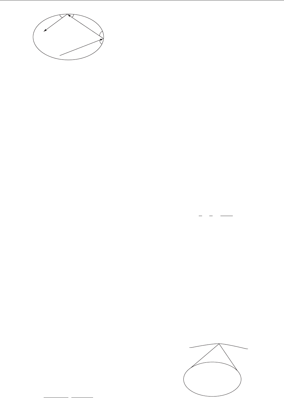
Equivalently, and more in the spirit of geometrical

optics, one considers L, the space of oriented

geodesics (rays of light) that intersect the billiard

table. This space of lines is in one-to-one correspon-

dence with the phase space of the billiard ball map:

to an inward unit vector (x, v) there corresponds the

oriented line through x in the direction v (Figure 1).

The space of rays L carries a canonical symplec-

tic structure, that is, a closed nondegenerate

differential 2-form. In the Euclidean case, this

symplectic structure ! is defined as follows. Given

an oriented line ‘ in R

, let q be the unit vector

along ‘ and p be the vector obtained by dropping

the perpendicular from the origin to ‘. Then,

! = dp ^ dq =

^ dq

. This construction identi-

fies L with the cotangent bundle of the unit sphere:

q is a unit vector and p is a (co)tangent vector at q,

and ! identifies with the canonical symplectic

structure of T



n1

. In the general case of a

Riemannian manifold M, the symplectic structure

on the space of oriented geodesics is obtained from

that on T



M by symplectic reduction.

One has an important result: the billiard ball map

preserves the symplectic structure T



(!) = !.Asa

consequence, T is also measure preserving. In the

planar case, one has the following explicit formula

for this measure. Let t be an arc length parameter

along the boundary of the billiard table and let

 2 [0, ] be the angle made by the unit vector with

this boundary. Then, (, t) are coordinates in the

phase space, identified with the cylinder, and the

invariant measure is sin  d dt.

As a consequence, the total area of the phase

space equals 2L where L is the perimeter length of

the boundary of the billiard table, and the mean free

path equals A=L, where A is the area of the billiard

table. In the general n-dimensional case, the mean

free path equals

volðS

n1

volðB

n1

volðMÞ

volð@MÞ

where S

n1

and B

n1

are the unit sphere and the unit

disk in Euclidean spaces.

Existence and Nonexistence of Caustics

Given a plane billiard table, a caustic is a curve

inside the table such that if a segment of a billiard

trajectory is tangent to this curve then so is each

reflected segment. Caustics correspond to invariant

circles of the billiard ball map (i.e., invariant curves

that go around the phase cylinder): such an invariant

circle is a one-parameter family of oriented lines,

and the respective caustic is their envelop. An

envelop may have cusp-like singularities but if the

boundary of the billiard table is a smooth curve with

positive curvature then a caustic, sufficiently close to

the boundary, is smooth and convex.

One can recover the table from a caustic by the

following string construction. Let  be a caustic.

Wrap a closed nonstretchable string around , pull it

tight at a point and move this point around  to

obtain a new curve . Then,  is a caustic for the

billiard inside . Note that this construction has one

parameter, the length of the string.

The following useful ‘‘mirror equation’’ relates

various quantities depicted in Figure 2:

sin 

where k is the curvature of the boundary at the

impact point.

Do caustics exist for every convex billiard table?

This is important to know, in particular, because the

existence of a caustic implies that the billiard ball

map is not ergodic. The answer is given by a

theorem of Lazutkin: if the boundary of the billiard

table is sufficiently smooth and its curvature never

vanishes, then there exists a collection of smooth

caustics in the vicinity of the billiard curve whose

union has a positive area. Originally this theorem

asked for 553 continuous derivatives; later this was

reduced to six. This result uses the techniques of the

KAM (Kolmogorov–Arnol’d–Moser) theory. The

Figure 1 Billiard ball map.

Figure 2 String construction and mirror equation.

Billiards in Bounded Convex Domains 297

crucial fact is that, in appropriate coordinates, the

billiard ball map is approximated, near the bound-

ary of the phase cylinder, by the integrable map

(x, y) 7!(x þ y, y).

On the other hand, by a theorem of Mather, if the

curvature of a convex smooth billiard curve vanishes

at some point, then this billiard ball map has no

invariant circles. This result belongs to the well-

developed theory of area-preserving twist maps of

the cylinder, of which the billiard ball map is an

example.

Integrable Billiards

Let a plane billiard table be an ellipse with foci F

and F

. It is known since antiquity that a billiard

ball shot from F

reflects to F

. A generalization of

this optical property of the ellipse is the following

theorem: a billiard trajectory inside an ellipse

forever remains tangent to a fixed confocal conic.

More precisely, if a segment of a billiard trajectory

does not intersect the segment F

, then all the

segments of this trajectory do not intersect F

and

are all tangent to the same ellipse with foci F

and F

;

and if a segment of a trajectory intersects F

then all the segments of this trajectory intersect F

and are all tangent to the same hyperbola with foci

and F

It follows that confocal ellipses are the caustics of

the billiard inside an ellipse. In particular, a

neighborhood of the boundary of such a billiard

table is foliated by caustics. A long-standing

conjecture, attributed to Birkhoff, asserts that if a

neighborhood of a strictly convex smooth boundary

of a billiard table is foliated by caustics, then this

table is an ellipse. This conjecture remains open. The

best result in this direction is a theorem of Bialy: if

almost every phase point of the billiard ball map in a

strictly convex billiard table belongs to an invariant

circle, then the billiard table is a disk.

The multidimensional analogs of the optical

properties of an ellipse are as follows. Consider an

ellipsoid M in R

given by the equation

þþ

¼1 ½1

and define the confocal family of quadrics M



by the

equation

þ 

þþ

þ 

¼ 1

where  is a real parameter. The topological type of



changes as  passes the values a

One has the following theorem: a billiard

trajectory inside M remains tangent to fixed

(n  1) confocal quadrics. A similar and closely

related result holds for the geodesic curves on M:

the tangent lines to a fixed geodesic on M are

tangent to (n  2) other fixed quadrics, confocal

with M. For a triaxial ellipsoid, this theorem goes

back to Jacobi.

Explicit formulas for the integrals of the billiard

in an n-dimensional ellipsoid [1] are as follows. Let

(x, v) be a phase point, a unit inward tangent vector

whose foot point x lies on the boundary. The

following functions are invariant under the billiard

ball map:

ðx; vÞ¼v

j6¼i

ðv

 v

 a

; i ¼ 1; ...; n

these functions are not independent: F

þþF

= 1.

In fact, the integrals F

Poisson-commute (with

respect to the Poisson bracket associated with the

symplectic structure in the phase space of the

billiard ball map that was described above). Accord-

ing to the Arnol’d–Liouville theorem, this complete

integrability of the billiard inside an ellipsoid implies

that the phase space is foliated by invariant tori and,

in appropriate coordinates, the map on each torus is

a parallel translation.

Similar results on complete integrability hold

for billiards inside quadrics in spaces of constant

positive or negative curvature. The former is

the intersection of a quadratic cone with the

unit sphere, and the latter with the unit

pseudosphere.

Periodic Orbits

Periodic billiard trajectories inside a planar billiard

table correspond to inscribed polygons of extremal

perimeter length. When counting periodic trajec-

tories, one does not distinguish between polygons

obtained from each other by cyclic permutation or

reversing the order of the vertices. In other words,

one counts the orbits of the dihedral group D

acting on n-periodic billiard polygons.

An additional topological characteristic of a

periodic billiard trajectory is the rotation number

defined as follows. Assume that the boundary  of a

billiard table is parametrized by the unit circle and

consider a polygon (x

, x

, ..., x

) inscribed in  .

For all i, one has x

i þ1

= x

þ t

with t

2 (0, 1). Since

the polygon is closed, t

þþt

2 Z. This integer,

that takes values from 1 to n  1, is called the

rotation number of the polygon and denoted by .

Changing the orientation of a polygon replaces the

298 Billiards in Bounded Convex Domains

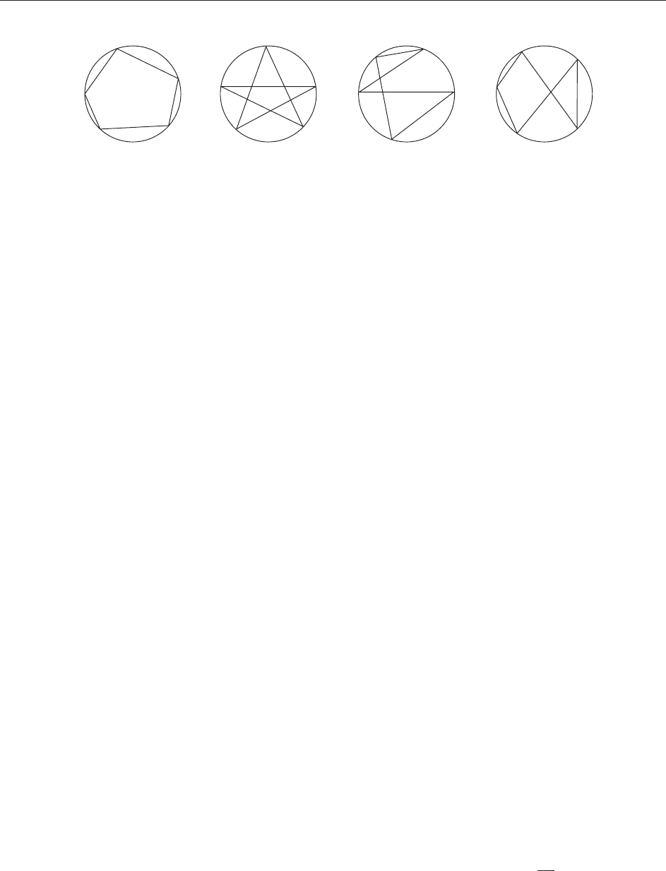
rotation number  by n  . The leftmost 5-periodic

trajectory in Figure 3 has  = 1 and the other three

 = 2.

The following theorem is due to Birkhoff: for

every n  2 and  b(n  1)= 2c , coprime with n,

there exist two geometrically distinct n-periodic

billiard trajectories with the rotation number . For

example, there are at least two 2-periodic billiard

trajectories inside every smooth oval: one is the

diameter, the longest chord, and another one is of

minimax type, similar to the minor axis of an

ellipse.

In higher dimensions, lower bounds on the

number of periodic billiard trajectories inside strictly

convex domains with smooth boundaries were

obtained only recently by Farber and the present

author. Here is one of the results: for a generic

billiard table in R

, the number of n-periodic

trajectories is not less than (n  1)(m  1). The

proof consists in using the Morse theory to estimate

below the number of critical points of the perimeter

length function on the space of inscribed n-gons and

its quotient space by the dihedral group D

, and the

main difficulty is in describing the topology of these

spaces.

Returning to convex smooth planar billiards, the

following conjecture remains open for a long time:

the set of n-periodic points of the billiard ball map

has zero measure. This is easy for n = 2; for n = 3

this is a theorem by M Rychlik. The motivation for

this question comes from spectral geometry. In

particular, according to a theorem of Ivrii, the

above conjecture implies the Weyl conjecture on

the second term for the spectral asymptotics of the

Laplacian in a bounded domain with the Dirichlet

or Neumann boundary conditions.

Length Spectrum

The set of lengths of the closed trajectories in a

convex billiard M is called the length spectrum of M.

There is a remarkable relation between the length

spectrum and the spectrum of the Laplace operator

in M with the Dirichlet boundary condition:

f = f , f j

= 0. From the physical point of view,

the eigenvalues  are the eigenfrequencies of the

membrane M with a fixed boundary. Roughly

speaking, one can recover the length spectrum from

that of the Laplacian. More precisely, the following

theorem of K Anderson and R Melrose holds:



2spec 

cos t

ﬃﬃﬃﬃﬃﬃﬃﬃ





is a well-defined generalized function (distribution)

of t, smooth away from the length spectrum. That is,

if l > 0 belongs to the singular support of this

distribution, then there exists either a closed billiard

trajectory of length l, or a closed geodesic of length l

in the boundary of the billiard table.

This relation between the Laplacian and the

length spectrum is due to the fact that geometric

optics is not a very accurate description of light. In

wave optics, light is considered as electromagnetic

waves, and geometric optics gives a realistic approx-

imation only when the wave length is small. This

small-wave approximation is based on the assump-

tion that the waves are locally almost harmonic,

while their amplitudes change slowly from point to

point. The substitution of such a function into the

corresponding PDEs gives, in the first approxima-

tion, the equations of wave fronts, that is, of

geometric optics.

Here is another spectral result concerning a

smooth strictly convex plane domain, due to

S Marvizi and R Melrose. Let L

be the supremum

and l

the infimum of the perimeters of simple

billiard n-gons. Then,

lim

n!1

ðL

 l

Þ¼0

for any positive k. Furthermore, L

has an asymp-

totic expansion, as n !1,

 l þ

i¼1

where l is the length of the boundary of billiard table

and c

are constants, depending on the curvature of

the boundary.

Figure 3 Rotation numbers of periodic trajectories.

Billiards in Bounded Convex Domains 299

Acknowledgments

This work was partially supported by NSF.

See also: Adiabatic Piston; Hamiltonian Systems:

Obstructions to Integrability; Hyperbolic Billiards;

Integrable Discrete Systems; Integrable Systems and

Algebraic Geometry; Optical Caustics; Integrable

Systems: Overview; Polygonal Billiards; Semiclassical

Spectra and Closed Orbits; Separatrix Splitting; Stability

Theory and KAM.

Further Reading

Chernov N and Markarian R, Theory of Chaotic Billiards

(to appear).

Farber M and Tabachnikov S (2002) Topology of cyclic

configuration spaces and periodic orbits of multi-dimensional

billiards. Topology 41: 553–589.

Gutkin E (2003) Billiard dynamics: a survey with the emphasis on

open problems. Regular and Chaotic Dynamics 8: 1–13.

Katok A and Hasselblatt B (1995) Introduction to the Modern

Theory of Dynamical Systems. Cambridge: Cambridge

University Press.

Kozlov V and Treshchev D (1991) Billiards. A Genetic Introduc-

tion to the Dynamics of Systems with Impacts. Providence:

American Mathematical Society.

Lazutkin V (1993) KAM Theory and Semiclassical Approxima-

tions to Eigenfunctions. Berlin: Springer.

Moser J (1980) Various Aspects of Integrable Hamiltonian Systems.

Progress in Mathematics, vol. 8, pp. 233–289. Basel: Birhauser.

Siburg KF (2004) The Principle of Last Action in Geometry and

Dynamics, Lecture Notes in Mathematics, vol. 1844. Berlin:

Springer.

Sinai Ya (1976) Introduction to Ergodic Theory. Princeton:

Princeton University Press.

Tabachnikov S (1995) Billiards, Socie´te´ Math. de France,

Panoramas et Syntheses, No 1.

Tabachnikov S (2005) Geometry and Billiards. American Mathe-

matic Society (to appear).

Black Hole Mechanics

A Ashtekar, Pennsylvania State University,

University Park, PA, USA

Introduction

Over the last 30 years, black holes have been

shown to have a number of surprising properties.

These discoveries have revealed unforeseen relations

between the otherwise distinct areas of general

relativity, quantum physics, and statistical

mechanics. This interplay, in turn, led to a number

of deep puzzles at the very foundations of physics.

Some have been resolved while others continue to

baffle physicists. The starting point of these

fascinating developments was the discovery of

laws of black hole mechanics by Bardeen,

Bekenstein, Carter, and Hawking. They dictate the

behavior of black holes in equilibrium, under small

perturbations away from equilibrium, and in fully

dynamical situations. While they are consequences

of classical general relativity alone, they have a

close similarity with the laws of thermodynamics.

The origin of this seemingly strange coincidence lies

in quantum physics. For further discussion,

see Asymptotic Structure and Conformal Infinity;

Loop Quantum Gravity; Quantum Geometry and

Its Applications; Quantum Field Theory in Curved

Spacetime; Stationary Black Holes.

The focus of this article is just on black hole

mechanics. The discussion is divided into three parts.

In the first, we will introduce the notions of event

horizons and black hole regions and discuss properties

of globally stationary black holes. In the second, we

will consider black holes which are themselves in

equilibrium but in surroundings which may be time

dependent. Finally, in the third part, we summarize

what is known in the fully dynamical situations. For

simplicity, all manifolds andfieldsareassumedtobe

smooth and, unless otherwise stated, spacetime is

assumed to be four dimensional, with a metric of

signature , þ , þ , þ , and the cosmological con-

stant is assumed to be zero. An arrow under a

spacetime index denotes the pullback of that index to

the horizon.

Global Equilibrium

To capture the intuitive notion that black hole is a

region from which signals cannot escape to the

asymptotic part of spacetime, one needs a precise

definition of future infinity. The standard strategy is to

use Penrose’s conformal boundary J

.Ablackhole

region B of a spacetime (M, g

)isdefinedasB = Mn



), where I



denotes ‘‘chronological past.’’ The

boundary @B of the black hole region is called the

‘‘event horizon’’ and denoted by E.Thus,E is the

boundary of the past of J

. It therefore follows that E is

a null 3-surface, ruled by future inextendible null

geodesics without caustics. If the spacetime is globally

hyperbolic, an ‘‘instant of time’’ is represented by a

Cauchy surface M. The intersection of B with M may

have several disjoint components, each representing a

black hole at that instant of time. If M

is a Cauchy

surface to the future of M, the number of disjoint

components of M

[ B in the causal future of M [ B

must be less than or equal to those of M [ B

300 Black Hole Mechanics

(see Hawking and Ellis (1973)). Thus, black holes can

merge but can not bifurcate. (By a time reversal, i.e., by

replacing J

with J



and I



with I

, one can define a

whiteholeregionW. However, here we will focus only

on black holes.)

A spacetime (M, g

) is said to be stationary (i.e., time

independent) if g

admits a Killing field t

that

represents an asymptotic time translation. By conven-

tion, t

is assumed to be unit at infinity. (M, g

)issaid

to be axisymmetric if g

admits a Killing field 

generating an SO(2) isometry. By convention 

normalized such that the affine length of its integral

curves is 2. Stationary spacetimes with nontrivial Mn



) represent black holes which are in global

equilibrium. In the Einstein–Maxwell theory in four

dimensions, there exists a unique three-parameter

family of stationary black hole solutions, generally

parametrized by mass m, angular momentum J,and

electric charge Q. This is the celebrated Kerr–Newman

family. Therefore, in general relativity a great deal of

work on black holes has focused on these solutions and

perturbations thereof. The Kerr–Newman family is

axisymmetric and furthermore, its metric has the

property that the 2-flats spanned by the Killing fields

and 

are orthogonal to a family of 2-surfaces. This

property is called ‘‘t– orthogonality.’ ’ These features of

Kerr–Newman space-times are widely used in black

hole physics. Note however that uniqueness fails in

higher dimensions, and also in the presence of

nonabelian gauge fields or rings of perfect fluids around

black holes in four dimensions. In mathematical

physics, there is significant literature on the new

stationary black hole solutions in Einstein–Yang–

Mills–Higgs theories. These are called ‘ ‘hairy black

holes.’’ Research on stationary black hole solutions with

rings received a boost by a recent discovery that these

black holes can violate the Kerr inequality J  Gm

between angular momentum J and mass m.

A null 3-manifold K in M is said to be a ‘‘Killing

horizon’’ if g

admits a Killing field K

which is

everywhere normal to K. On a Killing horizon, one

can show that the acceleration of K

is proportional

to K

itself:

¼ K

½1

The proportionality function  is called ‘‘surface

gravity.’’ We will show in the next section that if a

mild energy condition holds on K, then  must be

constant. Note that if we rescale K

via K

!cK

where c is a constant, surface gravity also rescales as

 !c.

In the Kerr–Newman family, the event horizon is

a Killing horizon. More generally, if an axisym-

metric, stationary black hole spacetime (M, g

)

satisfies the t– orthogonality property, its event

horizon E is a Killing horizon. (Although one can

envisage stationary black holes in which these

additional symmetry conditions are not met, this

possibility has been ignored in black hole mechanics

on stationary spacetimes. Quasilocal horizons, dis-

cussed below, do not require any spacetime symme-

tries.) In these cases, the normalization freedom in

is fixed by requiring that K

have the form

¼ t

þ 

½2

on the horizon, where  is a constant, called the

‘‘angular velocity of the horizon.’’ The resulting  is

called the surface gravity of the black hole. It is

remarkable that  is constant for all such black

holes, even when their horizon is highly distorted

(i.e., far from being spherically symmetric) either

due to rotation or due to external matter fields. This

is analogous to the fact that the temperature of a

thermodynamical system in equilibrium is constant,

independently of the details of the system. In

analogy with thermo dynamics, constancy of  is

referred to as the ‘‘zeroth law of black hole

mechanics.’’

Next, let us consider an infinitesimal perturbation

 within the three-parameter Kerr–Newman family.

A simple calculation shows that the changes in the

Arnowitt–Deser–Misner (ADM) mass m, angular

momentum J, and the total charge Q of the

spacetime and in the area a of the horizon are

constrained via

m ¼



8G

a þ   J þ Q ½3

where the coefficients , ,  are black hole para-

meters, =A

being the electrostatic potential at

the horizon. The last two terms, J and Q, have

the interpretation of ‘‘work’’ required to spin the

black hole up by an amount J or to increase its

charge by Q. Therefore, [3] has a striking resem-

blance to the first law, E = TS þ W, of thermo-

dynamics if (as the zeroth law suggests)  is made

proportional to the temperature T, and the horizon

area a to the entropy S. Therefore, [3] and its

generalizations discussed below are referred to as

the ‘‘first law of black hole mechanics.’’

In Kerr–Newman spacetimes, the only contribu-

tion to the stress–energy tensor come s from the

Maxwell field. Bardeen et al. (1973) consider

stationary black holes with matter such as perfect

fluids in the exterior region and stationary perturba-

tions  thereof. Using Einstein’s equations, they

show that the form [3] of the first law does not

change; the only modification is addition of certain

matter terms on the right-hand side which can be

Black Hole Mechanics 301

interpreted as the work W done on the total

system. A generalization in another direction was

made by Iyer and Wald (1994) using Noether

currents. They allow nonstationary perturbations

and, more importantly, drop the restriction to

general relativity. Instead, they consider a wide

class of diffeomorphism-invariant Lagrangian

densities L(g

, R

abcd

, r

bcde

, ..., 

, r



, ...)

which depend on the metric g

, matter fields 

and a finite number of derivatives of the Riemann

tensor and matter fields. Finally, they restrict

themselves to  6¼ 0. In this case, on the maximal

analytic extension of the spacetime, the Killing field

vanishes on a 2-sphere S

called the bifurcate

horizon. Then, [3] is generalized to

m ¼



2

S

hor

þ W ½4

Here W again represents ‘‘work terms’’ and S

hor

given by

hor

¼2

L

R

abcd

½5

where n

is the binormal to S

(with n

= 2),

and the functional derivative inside the integral is

evaluated by formally viewing the Riemann tensor

as a field independent of the metric. For the

Einstein–Hilbert action, this yields S

hor

= a=4 G and

one recovers [3].

These results are striking. However, the under-

lying assumptions have certain unsatisfactory

aspects. First, although the laws are meant to refer

just to black holes, one assumes that the entire

spacetime is stationary. In thermodynamics, by

contrast, one only assum es that the system under

consideration is in equilibrium, not the whole

universe. Second, in the first law, quantities a, , 

are evaluated at the horizon while M, J are

evaluated at infinity and include contributions from

possible matter fields outside the black hole. A more

satisfactory law of black hole mechanics would

involve attributes of the black hole alone. Finally,

the notion of the event horizon is extremely global

and teleological since it explicitly refers to J

.An

event horizon may well be developing in the very

room you are sitting today in anticipation of a

gravitational collapse in the center of our galaxy

which may occur a billion years hence. This feature

makes it impossible to generalize the first law to

fully dynamical situations an d relate the change in

the event horizon area to the flux of energy and

angular momentum falling across it. Indeed, one can

construct explicit examples of dynamical black holes

in which an event horizon E forms and grows in the

flat part of a spacetime where nothing happens

physically. These considerations call for a replace-

ment of E by a quasilocal horizon which leads to a

first law involving only horizon attributes, and

which can grow only in response to the influx of

energy. Such horizons are discussed in the next two

sections.

Local Equilibrium

The key idea here is drop the requirement that

spacetime should admit a stationary Killing field and

ask only that the intrinsic horizon geometry be time

independent. Consider a null 3-surface  in a

spacetime (M, g

) with a future-pointing normal

field ‘

. The pullback q

:= g

of the spacetime

metric to  is the intrinsic, degenerate ‘‘metric’’ of 

with signature 0, þ , þ . The first condition is that it

be ‘‘time independent,’’ that is, L

‘

= 0on.

Then by restriction, the spacetime derivative opera-

tor r induces a natural derivative operator D on .

While D is compatible with q

, that is, D

= 0, it

is not uniquely determined by this property because

is degenerate. Thus, D has extra information,

not contained in q

. The pair (q

, D) is said to

determine the intrinsic geometry of the null surface

. This notion leads to a natural definition of a

horizon in local equilibrium. Let  be a null, three-

dimensional submanifold of (M, g

) with topology

S  R, where S is compact and without boundary.

Definition 1  is said to be ‘‘isolated horizon’’ if it

admits a null normal ‘

such that:

(i) L

‘

= 0 and [L

‘

, D] = 0on and

(ii) T

‘

is a future pointing causal vector on .

On can show that, generically, this null normal field

‘

is unique up to rescalings by positive constants.

Both conditions are local to . In particular, (M, g

)

is not required to be asymptotically flat and there is no

longer any teleological feature. Since  is null and

‘

= 0, the area of any of its cross sections is the

same, denoted by a



. As one would expect, one can

show that there is no flux of gravitational radiation or

matter across . This captures the idea that the black

hole itself is in equilibrium. Condition (ii) is a rather

weak ‘‘energy condition’’ which is satisfied by all

matter fields normally considered in classical general

relativity. The nontrivial condition is (i). It extracts

from the notion of a Killing horizon just a ‘‘tiny part’’

that refers only to the intrinsic geometry of .Asa

result, every Killing horizon K is, in particular, an

isolated horizon. However, a spacetime with an

isolated horizon  can admit gravitational radiation

and dynamical matter fields away from . In fact, as a

family of Robinson–Trautman spacetimes illustrates,

302 Black Hole Mechanics

gravitational radiation could even be present arbitra-

rily close to . Because of these possibilities, there are

many nontrivial examples and the transition from

event horizons of stationary spacetimes to isolated

horizons represents a significant generalization of

black hole mechanics. (In fact, the derivation of the

zeroth and the first law requires slightly weaker

assumptions, encoded in the notion of a ‘‘weakly

isolated horizon’ ’ (Ashtekar et al. 2000, 2001).)

An immediate consequence of the requirement

‘

= 0 is that there exists a 1-form !

on  such

that D

‘

= !

‘

. Following the definition of  on a

Killing horizon, the surface gravity 

(‘)

of (, ‘)is

defined as 

(‘)

= !

‘

. Again, under ‘

!c‘

, we have



(c‘)

= c

‘

. Together with Einstein’s equations, the

two conditions of Definition 1 imply L

‘

= 0 and

‘

= 0. The Cartan identity relating the Lie

and exterior derivative now yields

ð!

‘

ÞD



ð‘Þ

¼ 0 ½6

Thus, surface gravity is consta nt on every isolate d

horizon. This is the zeroth law, extended to horizons

representing local equilibrium. In the presence of an

electromagnetic field, Definition 1 and the field

equations imply L

‘

= 0 and ‘

= 0. The first of

these equations implies that one can always choose a

gauge in which L

‘

= 0. By Cartan identity it then

follows that the electrostatic potential 

(‘)

:= A

‘

constant on the horizo n. This is the Maxwell analog

of the zeroth law.

In this setting, the first law is derived using a

Hamiltonian framework (Ashtekar et al. 2000,

2001). For concreteness, let us assume that we are

in the asymptotically flat situation and the only

gauge field present is electromagnetic. One begins by

restricting oneself to horizon geometries such that 

admits a rotational vector field ’

satisfying

’

= 0. (In fact for black hole mechanics, it

suffices to assume only that L

’



= 0, where 

the intrinsic area 2-form on . The same is true on

dynamical horizons discussed in the next section.)

One then constructs a phase space G of gravitational

and matter fields such that (1) M admits an internal

boundary  which is an isolated horizon; and (2) all

fields satisfy asymptotically flat boundary conditions

at infinity. Note that the horizon geometry is

allowed to vary from one phase-space point to

another; the pair (q

, D) induced on  by the

spacetime metric only has to satisfy Definition 1 and

the condition L

’

= 0.

Let us begin with angular momentum. Fix a

vector field 

on M which coincides with the fixed

’

on  and is an asymptotic rotational symmetry

at infini ty. (Note that 

is not restricted in any way

in the bulk.) Lie derivatives of gravitational and

matter fields along 

define a vector field X()on

G. One shows that it is an infinitesimal canonical

transformation, that is, satisfies L

X()

W = 0, where W

is the symplectic structure on G . The Hamiltonian

H() generating this can onical transformation is

given by

HðÞ¼J

ðÞ



 J

ðÞ



¼

8G

ð!



Þ 

4

ðA



½7

where J

()

is the ADM angular momentum at

infinity, S is any cross section of ,and the area

element thereon. The term J

()



is independent of the

choice of S made in its evaluatio n and interpreted as

the ‘‘horizon angular momentum.’’ It ha s numerous

properties that support this interpretation. In parti-

cular, it yields the standard angular momentum

expression in Kerr–Newman spacetimes.

To define horizon energy, one has to introduce a

‘‘time-translation’’ vector field t

. At infinity, t

must

tend to a unit time translation. On , it must be a

symmetry of q

. Since ‘

and ’

are both horizon

symmetries, t

= c‘

þ ’

on , for some constants

c and . However , unlike 

, the restriction of t

 cannot be fixed once and for all but must be

allowed to vary from one phase-space point to

another. In particular, on physical grounds, one

expects  to be zero at a phase-space point

representing a nonrotating black hole but nonzero

at a point representing a rotating black hole. This

freedom in the boundary value of t

introduces a

qualitatively new element. The vector field X(t)onG

defined by the Lie derivatives of gravitational and

matter fields does not, in general, satisfy L

X(t)

W = 0;

it need not be an infinitesimal canonical transforma-

tion. The necessary and sufficient condition is that

(

(c‘)

=8G)a



þ J



þ 

(c‘)

Q



be an exact var-

iation. That is, X(t) generates a Hamiltonian flow if

and only if there exists a function E

(t)



on G such that

E

ðtÞ



ðc‘Þ

8G

a



þ J



þ 

ðc‘Þ

Q



½8

This is precisely the first law. Thus, the framework

provides a deeper insight into the origin of the first

law: it is the necessary and sufficient condition for

the evolution generated by t

to be Hamiltonian.

Equation [8] is a genuine restriction on the choice of

phase-space functions c an d , that is, of restrictions

to  of evolution fields t

. It is easy to verify that M

admits many such vector fie lds. Given one, the

Hamiltonian H(t) generating the time evolution

along t

takes the form

HðtÞ¼E

ðtÞ

 E

ðtÞ



½9

Black Hole Mechanics 303

re-enforcing the interpretation of E

(t)



as the horizon

energy.

In general, there is a multitude of first laws, one for

each vector field t

, the evolution along which preserves

the symplectic structure. In the Einstein–Maxwell

theory, given any phase-space point, one can choose a

canonical boundary value t

exploiting the uniqueness

theorem. E

)



is then called the horizon mass and

denoted simply by m



.IntheKerr–Newmanfamily,

H(t

) vanishes and m



coincides with the ADM mass

. Similarly, if 

is chosen to be a global rotational

Killing field, J

()



equals J

()

. However, in more general

spacetimes where there is matter field or gravitational

radiation outside , these equalities do not hold; m



and J



represent quantities associ ated with the

horizon alone while the ADM quantities represent

the total mass and angular momentum in the space-

time, including contributions from matter fields and

gravitational radiation in the exterior region. In the

first law [8], only the contributions associated with

the horizon appear.

When the uniq ueness theorem fails, as, for

example, in the Einstein–Yang –Mills–Higgs theory,

first laws continue to hold but the horizon mass m



becomes ambiguous. Interestingly, these ambiguities

can be exploited to relate properties of hairy black

holes with those of the corresponding solitons. (For

a summary, see Ashtekar and Krishnan (2004).)

Dynamical Situations

A natural question now is whether there is an analog of

the second law of thermodynamics. Using event

horizons, Hawking showed that the answer is in the

affirmative (see Hawking and Ellis (1973)). Let (M, g

)

admit an event horizon E.Denoteby‘

a geodesic null

normal to E. Its expansion is defined as 

(‘)

:= q

‘

where q

is any inverse of the degenerate intrinsic

metric q

on E, and determines the rate of change of the

area element of E along ‘

. Assuming that the null energy

condition and Einstein’s equations hold, the Raychaud-

huri equation immediately implies that if 

(‘)

were to

become negative somewhere it would become infinite

within a finite affine parameter. Hawking showed that,

if there is a globally hyperbolic region containing



) [E– that is, if there are no naked singularities

– this can not happen, whence (‘)  0onE. Hence, if a

cross section S

of E is to the future of a cross section S

we must have a

 a

. Thus, in any (i.e., not

necessarily infinitesimal) dynamical process, the change

a in the horizon area is always non-negative. This

result is known as the ‘ ‘second law of black hole

mechanics.’’ As in the first law, the analog of entropy is

the horizon area.

It is tempting to ask if there is a local physical

process directly responsible for the growth of area.

For event horizons, the answer is in the negative

since they can grow in a flat portion of spacetime.

However, one can introduce quasilocal horizons

also in the dynamical situations and obtain the

desired result (Ashtekar and Krishnan 2003). These

constructions are strong ly motivated by earlier ideas

introduced by Hayward (1994).

Definition 2 A three-dimensional spacelike sub-

manifold H of (M, g

) is said to be a ‘‘dynamical

horizon’’ if it admits a foliation by compact

2-manifolds S (without boundary) such that:

(i) the expansion 

(‘)

of one (future directed) null

normal field ‘

to S vanishes and the expansion

of the other (future directed) null normal field,

is negative; and

(ii) T

‘

is a future pointing causal vector on H.

One can show that this foliation of H is unique and

that S is either a 2-sphere or, under degenerate and

physically over-restrictive conditions, a 2-torus. Each

leaf S isamarginallytrappedsurfaceandreferredtoasa

‘‘cut’’ of H. Unlike event horizons E, dynamical horizons

Hare locally defined and do not display any teleological

feature. In particular, they cannot lie in a flat portion of

spacetime. Dynamical horizons commonly arise in

numerical simulations of evolving black holes as world

tubes of apparent horizons. As the black hole settles

down, H asymptotes to an isolated horizon ,which

tightly hugs the asymptotic future portion of the event

horizon. However, during the dynamical phase, H

typically lies well inside E.

The two conditions in Definition 2 immediately

imply that the area of cuts of H increases mono-

tonically along the ‘‘outward direction’’ defined by

the projection of ‘

on H. Furthermore, this change

turns out to be directly related to the flux of energy

falling across H. Let R denote the ‘‘radius function’’

on H so that the area of any cut S is given by

= 4R

. Let N denote the norm of @

R and H,

the portion of H bounded by two cross sections S

and S

. The appropriate energy turns out to be

associated with the vector field N‘

, where ‘

normalized such that its projection on H is the unit

normal

to the cuts S. In the generic and

physically interesting case when S is a 2-sphere, the

Gauss and the Codazzi (i.e. , constraint ) equations

imply

ðR

R

Þ¼

H

N‘

^

V þ

16G



H

N 



þ2





V ½10

304 Black Hole Mechanics