Francoise J.-P., Naber G.L., Tsun T.S. (editors) Encyclopedia of Mathematical Physics
Подождите немного. Документ загружается.


weak gravity is in the locality of Earth. However, as
befits anything of Einsteinian nature, the weakness
of gravity is relative, so that at the surface of a
neutron star, one would find
R
M
R
0:4 ½3
while for black holes, one has
R
M
R
¼ 1 ½4
In such circumstances, gravity is anything but
weak! Furthermore, in situations where the mat-
ter–energy distribution has a highly time-dependent
quadrupole moment – such as occurs naturally with
a compact-binary system (i.e., a gravitationally
bound two-body system, in which each of the
bodies is either a black hole or a neutron star) – the
dynamics of the gravitational field, including,
crucially, the dynamics of the radiative components
of the gravitational field, can be expected to
dominate the dynamics of the overall system,
matter included. For scenarios such as these, it
should come as no surprise that the solution of the
combined gravitohydrodynamical system begs for
numerical analysis.
In addition, both from the physical and mathe-
matical perspectives, it is also natural to study the
strong, field dynamic regi mes (R !R
M
and/or v !c,
where v is the typical speed characterizing internal
bulk motion of the matter) of general relativity
within the context of a variety of matter models.
Typical processes addressed by these theoretical
studies include the process of black hole formation,
end-of-life events for various types of model stars,
and, again, the inte raction, including collisions, of
gravitationally compact objects. Note that it is
another hallmark of general relativity that highly
dynamical spacetimes need not contain any matter;
indeed, the interaction of two black holes – the
natural analog of the Kepler problem in relativity –
is a vacuum problem; that is, it is described by a
solution of [1] with T
= 0.
Motivated in significant part by the large-scale
efforts currently underway to directly detect gravita-
tional radiation (gravitational waves), much of the
contemporary work in numerical relativity is
focused on precisely the problem of the late phases
of compact-binary inspiral and merger. Such bin-
aries are expected to be the most likely candidates
for early detection by existing instruments such as
TAMA, GEO, VIRGO, LIGO, and, more likely, by
planned detectors including LIGO II and LISA (see,
e.g., Hough and Rowan (2000)). Detailed and
accurate predictions of expected waveforms from
these events – using the techniques of numerical
relativity – have the potential to substantially hasten
the discovery process, on the basis of the general
principle that if one knows what signal to look for,
it is much easier to extract that signal from the
experimental noise.
The computational task facing numerical relati-
vists who study problems such as binary inspiral is
formidable. In particul ar, such problems are intrin-
sically ‘‘3D,’’ to use the CFD (computational fluid
dynamics) nomenclature in which time dependence
is always assumed. That is, the PDEs that must be
solved govern functions, F(t, x
k
), that depend on all
three spatial coordinates, x
k
, as well as on time, t.
Unfortunately, even a cursory description of 3D
work in numerical relativity as it stands at this time
is far beyond the scope of this article.
What follows, then, is an outline of a traditi onal
approach to numerical relativity that underpins
many of the calculations from the early years of
the f ield (1970s and 1980s), most of which were
carried out with simplifying restrictions to
either spherical symmetry or axisymmetry. The
mathematical development, which will hereafter be
called the 3 þ 1 approach to general relativity, has
the advantage of using tensors and a n associated
tensor calculus that are reasonably intuitive for the
physicist. This ‘‘standard’’ 3 þ 1 approach is also
sufficient in many instances (particularly those
with symmetry) in the sense that i t leads to well-
posed sets of PDEs that can be discretized and
then solved computationally in a convergent
(stable) fashion. In addition, a thorough under-
standing of the 3 þ 1 approach will be of sig-
nificant help to the reader wishing to study any of
the c urrent literature in numerical relativity,
including the 3D w ork.
However, the reader is strongly cautioned that
the blind application of any of the equations that
follow, especially in a 3D context, may well lead
to ‘‘ill-posed systems,’’ numerical analysis of which
is useless. Anyone specifically interested in using
the m ethods of numerical relativity to generate
discrete, approximate solutions to [1],particularly
in the generic 3D c ase, is thu s urged to first
consult one of the comprehensive reviews of
numerical relativity that co ntinue to appear at
fairly regular intervals (see, e.g., Lehner (2001) ,or
Baumgarte and Shapiro (2003)). Most such refer-
ences will also provide a useful overview of many
of the most po pular numerical techniques that are
currently being used to discretize (convert to
algebraic form) the Einstein equations, as well as
the main algorithms that are used to solve the
resulting discrete e quations. These subjects are not
Computational Methods in General Relativity: The Theory 605

described below, not least sin ce discussion of the
available discretization techniq ues only makes
sense in the context of PDEs of specific systems
with specific boundary conditions, while there is
only space here to describe the general mathema-
tical setting for 3 þ 1 numerical relativity.
The 3 þ 1 Spacetime Split
At least at the current time, computations in
numerical relativity are restricted to the case of
globally hyperbolic spacetimes. A spacetime (four-
dimensional pseudo-Riemannian manifold), M
,
endowed with a metric, g
, is globally hyperbolic
if there is at least one edgeless, spacelike hypersur-
face, (0), that serve s as a Cauchy surface. That is,
provided that the initial data for the gravitational
field are set consistently on (0) – so that the four
constraint equations are satisfied (see below) – the
entire metric g
(t, x
i
) can be determined from the
field equations [1] (with appropriate boundary
conditions), and thus, so can the complete geometric
structure of the spacetime mani fold.
To be sure, global hyperbolicity is restrictive. It
excludes, for example, the highly interesting Go¨ del
universe. However, particularly from the point
of view of studying asymptotically flat solutions
(or solutions asymptotic to an y of the currently
popular cosmologies), as is usually the case in
astrophysics, the requirement of global hyperbolicity
is natural.
The 3 þ 1 split is based on the complete foliation
of M
based on level surfaces of a scalar function,
t – the time function. That is, the t = const. slices,
are three-dimensional spacelike (Riemannian) hyper-
surfaces, and, as t ranges from 1 to þ1,
completely fill the spacetime manifold, M
.In
order for the (t) to be everywhere spacelike,
t must be everywhere timelike:
g
r
tr
t < 0 ½5
Here r
is the spacetime covariant derivative
operator compat ible with the four metric, g
, thus
satisfying r
g
= 0, and g
is the inverse metric
tensor, which satisfies g
g
=
. The reader is
reminded that
is a Kronecker delta symbol; that
is,
has the value 1 if = , and the value 0
otherwise.
Furthermore, the scalar function t is now adopted
as the temporal coordinate, so that x
= (t, x
i
),
where the x
i
are the three spatial coordinates. As
noted implicitly above, since the problem under
consideration is a pure Cauchy evolution, the range
of t should nominally be infinite, both to the future
as well as to the past; that is, the solution domain is
1 < t < 1½6
jXj
ij
x
i
x
j
1=2
< 1½7
However, this assumes that one has global
existence for arbitrarily strong initial data, which
is decidedly not always the case in general
relativity. Indeed, ‘‘continued’’ or ‘‘catastrophic’’
gravitational collapse – that is, the process of black
hole formation – signaled, in modern language, by
the appearance of a trapped surface, inexorably
leads to a physical singularity, which – the
somewhat vague nature of the singul arity theorems
of Penrose, Hawking, and others notwithstanding –
in actual numerical computations invariably turns
out to be ‘‘catastrophic’’ in terms of Cauchy
evolution.
Such behavior in time-dependent nonlinear PDEs
is quite familiar in the mathematical community at
large, where it is frequently known as finite-time
blow-up (or finite-time singularity). However,
despite the fact that such behavior is one of the
most fascinating aspects of solutions of the Einstein
equations, the following discussion will be, impli-
citly at least, restricted to the case of weak initial
data, that is, to initial data for which there is global
existence.
With the manifold M
sliced into an infinite
stack of spacelike hypersurfaces, (t), attention
shifts to any single surface, as well as to the
manner in which such a generic surface is
embedded in the spacetime.
First, each spacelike hypersurface, (t), is itself a
three-dimensional Riemannian differential manifold
with a metric
ij
(t, x
k
). (Note that in this discussion,
the symbol t is to be understood to represent any
specific value of coordinate time.) From this metric,
one can construct an inverse metric,
ij
(t, x
k
),
defined, as usual, so that
ik
kj
¼
i
j
½8
Associated with the spatial metric,
ij
, is a natural
spatial covariant derivative operator, D
i
, that is
compatible with
ij
:
D
k
ij
¼ 0 ½9
With the spatial metric,
ij
, and its inverse,
ij
,in
hand, the standard formulas of tensor analysis can
be applied to compute the usual suite of geome-
trical tensors. All tensors thus computed, and
indeed, all tensors defined intrinsically to the
606 Computational Methods in General Relativity: The Theory
hypersurfaces (t) are called ‘‘spatial’’ tensors, and
have their indices (if any) raised and lowered with
ij
and
ij
, respectively.
Thus, the Christoffel symbols of the second kind,
i
jk
, are given by
i
jk
¼
1
2
il
@
k
lj
þ @
j
lk
@
l
jk
½10
Note that these quantities are symmet ric in their last
two indices
i
jk
¼
i
kj
½11
and that they can be used, as usual, in explicit
calculation of the action of the spatial covariant
derivative operator on an arbitrary tensor. In
particular, for the special cases of a spatial vector,
V
i
, and a covector (1-form), W
i
, one has
D
i
V
j
¼ @
i
V
j
þ
j
ik
V
k
½12
and
D
i
W
j
¼ @
i
W
j
k
ij
W
k
½13
respectively.
Given the Christoffel symbols, the components of
the spatial Riemmann tensor, denoted here R
ijk
l
, are
computed using
R
ijk
l
¼@
j
l
ik
@
i
l
jk
þ
m
ik
l
mj
m
jk
l
mi
½14
Finally, the Ricci tensor, R
i
j
, and Ricci scalar, R, are
defined in the usual fashion
R
i
j
¼
ik
R
kj
¼
ik
R
klj
l
½15
R¼
ij
R
ij
½16
The reader shou ld again note that all of the
tensors just defined ‘‘live’’ on each and every single
spacelike hypersurface, (t), and are thus known as
hypersurface-intrinsic quantities. In particular, the
spatial Riemann tensor, R
ijk
l
, which encodes all
intrinsic geometric information about (t), in no
way depends on how the slice is embedded in the
spacetime M
.
The next step in the 3 þ 1 app roach involves
rewriting the fundamental spacetime line element for
the squared proper distance, ds
2
, between two
spacetime events, P and Q, having coordinates x
and x
þ dx
, respectively,
ds
2
¼ g
dx
dx
½17
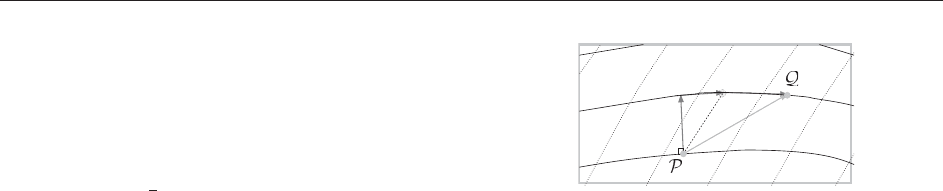
As Figure 1 illustrates, a quick route to the 3 þ 1
decomposition of the above expression, and thus of
the tensor g
itself, is based on an application of
the ‘‘four-dimensional Pythagorean theorem.’’ In
setting up the calculation, one naturally identifies
four functions, the scalar lapse, (t, x
k
), and the
vector shift,
i
(t, x
k
), that encode the full coordi-
nate (gauge) freedom of the theory. That is,
complete specification of the lapse and shift is
equivalent to completely fixing the spacetime
coordinate system.
In light of the above discussi on, and again
referring to Figure 1, one readily deduces the 3 þ 1
decomposition of the spacetime line element:
ds
2
¼
2
dt
2
þ
ij
dx
i
þ
i
dt
dx
j
þ
j
dt
½18
A rearranged form of this last expression is also
often seen in the literature:
ds
2
¼
2
þ
k
k
dt
2
þ 2
k
dx
k
dt
þ
ij
dx
i
dx
j
½19
The following useful identifications of the ‘‘time–
time,’’ ‘‘time–space,’’ and ‘‘space–space’’ pieces of
the spacetime metri c, g
, follow immediately from
[19]:
g
00
¼
2
þ
i
i
½20
g
0i
¼ g
i0
¼
i
¼
ik
k
½21
g
ij
¼
ij
½22
This last relation is an example of a useful general
result; the purely spatial components, Q
ijk
,ofa
α dt
β
i
dt
dx
i
dx
μ
Σ(t )
Σ(t
+ dt )
Figure 1 Spacetime displacement in the 3 þ 1 approach,
following Misner, Thorne, and Wheeler (1973). Solid lines represent
surfaces of constant time, t ; that is, each solid line represents a
single spacelike hypersurface, (t). Dotted lines denote trajectories
of constant spatial coordinate, that is, trajectories with x
k
= const.
The lapse function, (t, x
k
), encodes the (local) ratio between
elapsed coordinate time, dt, and elapsed proper time, d = dt,for
an observer moving normal to the slices (i.e., for an observer with a
4-velocity, u
, identical to the hypersurface normal, n
). Similarly,
the shift vector,
i
(t, x
k
), describes the shift,
i
(t, x
i
)dt,in
trajectories of constant spatial coordinate – the dotted lines in the
figure – relative to motion perpendicular to the slices. The 3 þ 1
form of the line element [18] then follows immediately from an
application of the spacetime version of the Pythagorean theorem.
Computational Methods in General Relativity: The Theory 607

completely covariant, but otherwise arbitrary, space-
time tensor, Q
, constitute the components of a
completely covariant spatial tensor.
A straightforward calculation, which provides a
good exercise in the use of the 3 þ 1 calculus,
yields the following equally useful identifications for
various pieces of the inverse spacetime metric: g
g
00
¼
2
½23
g
0i
¼ g
i0
¼
2
i
½24
g
ij
¼
ij
2
i
j
½25
Since the Einstein field equations are equations
with, loosely speaking, geometry on one side and
matter on the other, tensors built from matter fields
must also be decomposed. In particular, it is
conventional to defi ne tensors, , j
i
, and S
ij
that
result from various projections of the spacetime
stress energy tensor, T
, onto the hypersurface:
n
n
T
½26
j
i
n
T
i
½27
S
ij
T
ij
½28
For observers with 4-velocities u
equal to n
, and
only for those observers with u
= n
, the above
quantities have the interpre tation of the locally and
instantaneously measured energy density, momen-
tum density, and spatial stresses, respectively. As
with the geome tric quantities, all of the matter
variables, , j
i
, and S
ij
defined in [26]–[28] are
spatial tensors and thus have their indices (if any)
raised and lowered with the 3-metric. Note that the
identification S
ij
= T
ij
is another illustration of
the general result mentioned in the context of the
previous identification of
ij
and g
ij
.
Finally, observing that time parameters are natu-
rally defined in terms of level surfaces (equipotential
surfaces), it should be no surprise that the covariant
components, n
, of the hypersurface normal field,
n
¼; 0; 0; 0ðÞ ½29
are simpler than the components, n
, of the normal
itself,
n
¼
1
;
1
i
½30
and, in fact, eqn [29] can also be deduced from a
quick study of Figure 1.
In the 3 þ 1 approach, in addition to the 3-metric,
ij
(t, x
k
), and coordinate functions, (t, x
i
)and
(t, x
i
), it is convenient to introduce an additional
rank-2 symmetric spatial tensor, K
ij
(t, x
k
), known as
the extrinsic curvature (or second fundamental
form). This additional tensor is analogous to a
time derivative of
ij
(t, x
k
), or, from a Hamiltonian
perspective, to a variable that is dynamically
conjugate to
ij
(t, x
k
).
As the name suggests, the extrinsic curvature
describes the manner in which the slice (t)is
embedded in the manifold (to be contrasted with
R
ijk
l
defined by [14] which is, as mentioned
previously, completely insensitive to the manner in
which the hypersurface is embe dded in M
).
Geometrically, K
ij
is computed by calculating the
spacetime gradient of the normal covector field, n
,
and projecting the result on to the hypersurface,
K
ij
¼
1
2
r
i
n
j
½31
where it must be stresse d that r
is the spacetime
covariant derivative operator compatible with the
4-metric, g
; that is, r
g
= 0. A straightforward
tensor calculus calculation then yields the following,
which can be viewed as a definition of the K
ij
:
K
ij
¼
1
2
@
t
ij
þ D
i
j
þ D
j
i
½32
Here, D
i
is the spatial covariant metric, compatible
with
ij
(D
k
ij
= 0), that was defined previously.
Observe that this equation can be easily solved for
@
t
ij
(this will be done below), and thus, in the 3 þ 1
approach it is [32] that is the origin of the evolution
equations for the 3-metric components,
ij
.
Einstein’s Equations in 3 þ 1 Form
The Constraint Equations
As is well known, as a result of the coordinate (gauge)
invariance of the theory, general relativity is overdeter-
mined in a sense completely analogous to the situation
in electrodynamics with the Maxwell equations. One
of the ways that this situation is manifested is via the
existence of the constraint equations of general
relativity. Briefly, starting from the naive view that
the ten metric functions, g
(t, x
i
), that completely
determine the spacetime geometry are all dynamical –
that is, that they satisfy second-order-in-time equations
of motion – one finds that the Einstein equations do not
provide dynamical equations of motion for the lapse,
, or the shift,
i
. Rather, four of the field equations [1]
are equations of constraint for the ‘‘true’’ dynamical
variables of the theory, {
ij
, @
t
ij
}, or, equivalently,
{
ij
, K
i
j
}. Note that in the following, the mixed
form, K
i
j
, is at times used – again by convention – as
the principal representation of the extrinsic curvature
tensor (instead of K
ij
as previously, or K
ij
).
608 Computational Methods in General Relativity: The Theory

Thus, four of the components of [1] can be
written in the form
C
ij
; K
i
j
;@
k
ij
;@
l
@
k
ij
;@
k
K
i
j
¼T
½33
where T
depends only on the matter content in the
spacetime. Note that in addition to having no
dependence on @
2
t
ij
, the constraints are also
independent of and
i
.
If the Einstein equations [1] are to hold throughout
the spacetime, then the constraints [33] must hold on
each and every spacelike hypersurface, (t), including,
crucially, the initial hypersurface, (0). From the point
of view of Cauchy evolution, this means that the 12
functions, {
ij
(0, x
k
), K
i
j
(0, x
k
)}, constituting the grav-
itational part of the initial data, are not completely
freely specifiable, but must satisfy the four constraints
C
ij
ð0; x
k
Þ; K
i
j
ð0; x
k
Þ; ...
¼T
ð0; x
k
Þ½34
However, provided initial data that do satisfy the
equations is chosen, then – as consistency of the
theory demands – the dynamical equations of
motion for the {
ij
, K
i
j
}(eqns [37] and [38] below)
guarantee that the constraints will be satisfied on all
future (or past) hypersurfaces, (t). In this internal
self-consistency, the geometrical Bianchi identities,
r
G
= 0, and the local conservation of stress
energy, r
T
= 0, play crucial roles.
In the 3 þ 1 approach, as one would expect, the
constraint equations further naturally subdivide into
a scalar equation
RK
ij
K
ij
þ K
2
¼ 16 ½35
and a (spatial) vector equation
D
j
K
ij
D
i
K ¼ 8j
i
½36
where the energy and momentum densities, and j
i
=
ik
j
k
, are given by [26]–[28]. Equations [35] and [36]
are often known as the Hamiltonian and momentum
constraint, respectively, not least since the behavior of
their solutions as X
ffiffiffiffiffiffiffiffiffiffiffiffiffi
ij
x
i
x
j
p
!1 encodes the
conserved mass and linear momentum (four numbers)
that can be defined in asymptotically flat spacetimes.
In a general 3 þ 1 coordinate system, and with an
appropriate choice of variables, the constraints can
be written as a set of quasilinear elliptic equations
for four of the {
ij
, K
i
j
} (or, more properly, for
certain algebraic combinations of the {
ij
, K
i
j
}).
Thus, especially for 2D and 3D calculations, the
setting of initial data for the Cauchy problem in
general relativity is itself a highly nontrivial mathe-
matical and computational exercise. Readers
wishing more details on this subject are directed to
the comprehensive review by Cook (2000).
The Evolution Equations
As discussed above, in the 3 þ 1 form of the Einstein
equations [1], the spatial metric,
ij
, and the
extrinsic curvature, K
i
j
, are viewed as the dynamical
variables for the gravitational field. The remainder
of the 3 þ 1 equations are thus two sets of six first-
order-in-time evolution equations; one set for
ij
,
@
t
ij
¼2
ik
K
k
j
þ
k
@
k
ij
þ
ik
@
j
k
þ
kj
@
i
k
½37
and the other set for K
i
j
,
@
t
K
i
j
¼
k
@
k
K
i
j
@
k
i
K
k
j
þ@
j
k
K
i
k
D
i
D
j
þ R
i
j
þKK
i
j
þ8
1
2
i
j
S ðÞS
i
j
½38
As also noted previously, the evolution equa tions
[37] for the spatial metric compone nts,
ij
, follow
from the definition of the extrinsic curvature [31].
The derivation of the equations for the extrinsic
curvature, on the other hand, require lengthy, but
well-documented, manipulations of the spatial com-
ponents of the field equations [1].
The (Naive) Cauchy Problem
A naive statement of the Cauchy problem for 3 þ 1
numerical relativity is thus as follow s: fix a speci-
fied number, N, of matter fields
A
(t, x
k
), A =
1, 2, ..., N, all minimally coupled to the gravita-
tional field, with a total stress tensor, T
, given by
T
¼
X
N
A¼1
T
A
½39
where T
A
is the stress tensor correspo nding to the
matter field
A
. Choose a topolog y for (0) (e.g., R
3
with asymptotical ly flat boundary conditions; T
3
,
with no boundaries, etc.) This also fixes the
topology of M
to be Rthe topology of (0).
Next, freely specify eight of the 12 {
ij
(0, x
k
),
K
i
j
(0, x
k
)}, as well as initial values,
A
(0, x
k
), for the
matter fields. Then determine the remaining four
dynamical gravitational fields from the constraints
[35] and [36]. This completes the initial data
specification.
One must now choose a prescription for the
kinematical (coordinate) functions, and
i
,sothat
either explicitly or implicitly, they are completely fixed;
for the case of implicit specification, this may well
mean that the coordinate functions themselves will
satisfy PDEs, which, furthermore, can be of essentially
any type in practice (i.e., elliptic, hyperbolic, para-
bolic, ...). Finally, with consistent initial data,
{
ij
(0, x
k
), K
i
j
(0, x
k
);
A
(0, x
k
)}, in hand, and with a
prescription for the coordinate functions, the evolution
Computational Methods in General Relativity: The Theory 609

equations [37] and [38] canbeusedtoadvancethe
dynamical variables forward or backward in time.
The above description is naive since, apart from a
consistent mathematical specification, the most crucial
issue in the solution of a time-dependent PDE as a
Cauchy problem is that the problem be ‘‘well posed.’’
Roughly speaking, this means that solutions do not
grow without bound (‘‘blow-up’’) without physical
cause, and that small, smooth changes to initial data
yield correspondingly small, smooth changes to the
evolved data. In short, the Cauchy problem must be
stable, and whether or not a particular subset of
the equations displayed in this section yields a well-
posed problem is a complicated and delicate issue,
especially in the generic 3D case. The reader is thus
again cautioned against blind application of any of the
equations displayed in this article.
Boundary Conditions
In principle, because all spacelike hypersurfaces, (t),
in a pure Cauchy evolution are edgeless – and provided
that the initial data {
ij
(0, x
k
), K
i
j
(0, x
k
);
A
(0, x
k
)} is
consistent with asymptotic flatness, or whatever other
condition is appropriate given the topology of the
(t) – there are essentially no boundary conditions to
be imposed on the dynamical variables, {
ij
(t, x
k
),
K
i
j
(t, x
k
)}, during Cauchy evolution. Note that asymp-
totic flatness generally requires that
lim
X !1
ij
¼ f
ij
þ O
1
X
½40
and
lim
X!1
K
i
j
¼ O
1
X
2
½41
where X is defined by
X
ffiffiffiffiffiffiffiffiffiffiffiffiffi
ij
x
i
x
j
q
½42
as previously, and f
ij
is the flat 3-metric. Similarly,
should the lapse, , and shift, , be constrained by
elliptic PDEs – as is frequently the case in practice –
then the only natural place to set boundary condi-
tions is at spatial infinity, and then, provided that
the frame at spatial infinity is inerti al, with
coordinate time t measuri ng proper time, one should
have
lim
X !1
¼ 1 þ O
1
X
½43
and
lim
X !1
i
¼ O
1
X
½44
It is critical to note at this point, however, that in
the vast bulk of past and current work in numerical
relativity, including most of the ongoing work in
3D, the Einstein equations [1] have been solved, not
as a pure Cauchy problem, but as a mixed initial-
value/boundary-value (IBVP) problem. That is, in
the discretization process in which the continuum
equations [1] are replaced with algebraic equations,
the continuum domain [6]–[7] is typically replaced
with a truncated spatial domain
jx
i
jX
i
max
½45
where the X
i
max
are a priori specified constants
(parameters of the computational solution) that
define the extremities of the ‘‘computational box.’’
As one might expect, the theory underlying stability
and well-posedness of IBVP problems – especially
for differential systems as complicated as [1] –is
even more involved than for the pure initial-value
case, and is another very active area of research in
both mathematical and numerical relativity
(see, e.g., Friedrich and Nagy (1999 )).
See also: Critical Phenomena in Gravitational Collapse;
Einstein Equations: Initial Value Formulation; Fluid
Mechanics: Numerical Methods; General Relativity:
Overview; Geometric Analysis and General Relativity;
Gravitational Waves; Hamiltonian Reduction of Einstein’s
Equations; Magnetohydrodynamics; Spacetime
Topology, Causal Structure and Singularities; Symmetric
Hyperbolic Systems and Shock Waves.
Further Reading
Baumgarte T and Shapiro SL (2001) Numerical relativity and
compact binaries. Physics Reports 376: 41–131.
Cook G (2000) Initial data for numerical relativity. Living
Reviews of Relativity 3: 5 (irr-2000-5).
Font JA (2003) Numerical hydrodynamics in general relativity.
Living Reviews of Relativity 6: 4 (irr-2003-4).
Frauendiener J (2004) Conformal infinity. Living Reviews of
Relativity 7: 1 (irr-2004-1).
Friedrich H and Nagy G (1999) The initial boundary value
problem for Einstein’s vacuum field equation. Communica-
tions in Mathematical Physics 201: 619–655.
Hough J and Rowan S (2000) Gravitational wave detection by
interferometry (ground and space). Living Reviews of Rela-
tivity 3: 3 (irr-2000-3).
Lehner L (2001) Numerical relativity: a review. Classical and
Quantum Gravity 18: R25–R86.
Misner CW, Thorne KS, and Wheeler JA (1973) Gravitation.
San Francisco: W.H. Freeman.
Reula OA (1998) Hyperbolic methods for Einstein’s equations.
Living Reviews of Relativity 1: 3 (irr-1998-3).
Winicour J (2001) Characteristic evolution and matching. Living
Reviews of Relativity 4: 3 (irr-2001-3).
610 Computational Methods in General Relativity: The Theory

Confinement see Quantum Chromodynamics
Conformal Geometry see Two-dimensional Conformal Field Theory and Vertex Operator Algebras
Conservation Laws see Symmetries and Conservation Laws
Constrained Systems
M Henneaux, Universite
´
Libre de Bruxelles,
Brussels, Belgium
ª 2006 Elsevier Ltd. All rights reserved.
Introduction
Consider a dynamical system with coordinates
q
i
(i = 1, ..., n) and Lagrangian L(q
i
,
˙
q
i
) (field theory
is formally covered by regarding the spatial coordi-
nates as a continuous index). When going to the
Hamiltonian formulation, it is usually assumed that
the Legendre transformation between the velocities
˙
q
i
and the momenta
p
i
¼
@L
@
_
q
i
½1
can be inverted to yield the velocities as functions of
the q’s and the p’s. This ‘‘regular’’ situation occurs
for most systems appearing in standard classical
mechanics and enables one to proceed to the
Hamiltonian formulation of the theory without
difficulty.
In field theory, however, the regular case is the
exception rather than the rule. This is due to gauge
invariance and first-order Lagrangians.
Gauge invariance A system possesses gauge sym-
metries if it is invariant under transformations that
involve arbitrary functions of time (gauge trans-
formations). In that case, the solution of the
equations of motion with given initial data is not
unique, since it is always possible to perform a
gauge transformation in the course of the evolution
without changing the initial data. It is then clear
that the Legendre transformation cannot be inver-
tible, for if it were, one could rewrite the equations
of motion in the standard canonical form
˙
q
i
= @H=@p
i
,
˙
p
i
= @H=@q
i
. These canonical
equations are in normal form and have a unique
solution for given initial data, which would
contradict the presence of a gauge symmetry.
A simple example that illustrates this phenom-
enon is given by the following model for three
variables q
1
, q
2
, and , the Lagrangian of which
reads
L ¼
1
2
ð
_
q
1
Þ
2
þð
_
q
2
Þ
2
½2
This model is inspired by electromagnetism: the
variables q
1
and q
2
play a role somewhat similar
to that of the spatial components of the vector
potential, while corresponds to the temporal
component. The Lagrangian is invariant under the
gauge transformations
q
1
! q
1
þ "; q
2
! q
2
þ "; ! þ
_
" ½3
where " is an arbitrary function of time. The
conjugate momenta are
p
1
¼
_
q
1
; p
2
¼
_
q
2
;
¼ 0
One cannot invert the Legendre transformation
since one cannot express the velocity
_
in terms of
the momenta.
First-order Lagrangians Fermionic fields obey
first-order equations. Their Lagrangian is linear
in the derivatives, so that the conjugate momenta
p
i
depend on the coordinates q
i
only. It is then
clearly impossible to express the velocities in
terms of the momenta through the Legendre
transformation. More generally, any first-order
Lagrangian with or without gauge symmetry leads
to a noninvertible Legendre transformation.
Constrained Systems 611

A simple system that exhibits this feature is
described by the Lagrangian
L ¼ z
2
_
z
1
1
2
ðz
2
Þ
2
½4
for two bosonic degrees of freedom (z
1
, z
2
). This
is in fact the canonical form of the Lagrangian for
a free particle in one dimension (z
2
is the
momentum conjugate to the position z
1
): the
system is already in Hamiltonian form. There is
no gauge invariance, but because the Lagrangian
is first order, the Legendre transformation with
[4] as starting point,
p
1
¼ z
2
; p
2
¼ 0 ½5
is non invertible for the velocities (which do not
even appear in the formulas for the momenta).
Dirac showed how to develop the Hamiltoni an
formalism in the case when the Legendre transfor-
mation is not invertible. One can still reformulate
the equations in phase space and write them in terms
of brackets with the Hamiltonian, but a new major
feature emerges, namely the canonical variables are
no longer free. Rather, the permiss ible phase-space
points are constrained to be on the so-called
‘‘constrained surface.’’ For this reason, systems for
which the Legendre transformation is not invertible
are also called ‘‘constrained Hamiltonian systems.’’
We shall adopt this terminology here.
The purpose of this article is to explain the main
ideas underlying the Dirac method. To simplify the
discussions and to focus on the features peculiar to
the Dirac construction, we shall assume as a rule
that all necessary smoothness conditions are fulfilled
by the functions, surfaces, etc., appearing in the
formalism. How to develop the analysis when some
of the smoothness conditions are not fulfilled is of
definite interest but goes beyond the scope of this
review. We shall also assume, for definiteness, that
all the variables are bosonic in order to avoid
straightforward but somewhat cumbersom e sign
factors in the formulas.
General Theory
Dirac Algorithm
Primary constraints When the Legendre transfor-
mation [1] cannot be inverted, the momenta p
i
’s do
not span an n-dimensional space but are constrained
by relations
m
ðq; pÞ¼0; m ¼ 1; ...; M ½6
which follow from their definition. These equations
reduce to identities when the momenta are replaced
by their expression [1] in terms of the coordinates
and the velocities. They are called primary con-
straints. We shall assume that the matrix
@ð
m
Þ
@ðp
i
; q
i
Þ
is every where of constan t (maximum) rank M on the
phase-space surface defined by eqns [6] which is
assumed to be smooth. This surface is of dimensi on
2n M.
Canonical Hamiltonian The next step in the Dirac
procedure is to define the canonical Hamiltonian H
through
H ¼
_
q
i
p
i
L ½7
As shown by Dirac, H can be re-expressed as a
function H(q, p) of the momenta and the co ordi-
nates, even when the Legendre transformation is not
invertible: the canonical Hamiltonian H depends on
the velocities only through the p
i
’s. Furthermore, the
original equations of motion in Lagrangian form are
equivalent to the Hamiltonian equations
_
q
i
¼
@H
@p
i
þ u
m
@
m
@p
i
½8
_
p
i
¼
@H
@q
i
u
m
@
m
@q
i
½9
m
ðq; pÞ¼0 ½10
where the u
m
’s are parameters, some of which will
be determined through the consistency algorithm to
be discussed shortly. (In [7]–[9] and everywhere
below, there is a summation over the repeated
indices.)
Secondary constraints The equations of motion [8]
and [9] can be rewritten as
_
F ¼½F; Hþu
m
½F;
m
½11
where F = F(q, p) is any function of the canonical
variables. Here, the Poisson bracket is defined as
usual by
½G; F¼
@G
@q
i
@F
@p
i
@G
@p
i
@F
@q
i
½12
If one takes for F one of the primary constraints
m
, one should get zero,
_
m
= 0. This yields the
consistency conditions
½
m
; Hþu
m
0
½
m
;
m
0
¼0 ½13
These conditions can imply further restrictions on the
canonical variables and/or impose conditions on the
612 Constrained Systems

variables u
m
. Any new relation X(q, p) = 0onthe
canonical variables leads, in turn, to a further consis-
tency condition
˙
X = [X, H] þ u
m
0
[X,
m
0
] = 0, which
can bring in either further restriction on the constraint
surface or fix more variables u
m
. Constraints that
follow from the consistency algorithm are called
‘‘secondary constraints.’’ Finally, one is left with a
certain number of secondary constraints, which are
denoted by
k
= 0, k = M þ 1, ..., M þ K. We assume
again that all the constraints (primary and secondary)
define a smooth surface, called the ‘ ‘constraint surface,’’
and fulfill the condition that @(
k
)=@(q
i
, p
i
)isof
maximum rank J M þ K on the constraint surface.
(We also assume for simplicity that there is no
branching in the consistency algorithm.)
Restrictions on the u’s Having a complete set of
constraints
j
¼ 0; j ¼ 1; ...; M þ K J ½14
we can now investigate more precisely the restric-
tions on the variables u
m
. These read
½
j
; Hþu
m
½
j
;
m
0; j ¼ 1; ...; J ½15
where the notation means ‘‘equal modulo the
constraints.’’ In [15], m is summed from 1 to M.
Equations [15] are a set of J linear, inhomogeneous
equations for the u’s, with coefficients that are
functions of the canonical variables q
i
, p
i
. The
general solution of this system is of the form
u
m
¼ U
m
þ u
a
V
m
a
½16
where U
m
is a particular solution and where the V
m
a
(a = 1, ..., A) provide a complet e set of independent
solutions of the homogeneous system
V
m
a
½
j
;
m
0 ½17
The coefficients u
a
(a = 1, ..., A) are compl etely
arbitrary.
We thus see the emergence of another new feature
in the theory, in addition to the appearance of
constraints. It is that the general solution of the
equations of motion may contain arbitrary functions
of time (when A 6¼ 0), in agreement with the
possible presence of a gauge symmetry.
First- and Second-Class Constraints
First- and second-class functions A function F (q, p)
is called a first-class function if it generates a
canonical transformation that maps the constraint
surface on itself. Thus, F(q, p) is first class if its
Poisson brackets with all the constraints vanish
weakly (i.e., are zero on the constraint surface),
½F ;
j
0; j ¼ 1; ...; J ½18
A function is second class otherwise, that is, if there
is at least one constraint
j
such that [F,
j
] 6¼ 0
(not even weakly). Second- class functions generate
canonical transformations that do not leave the
constraint surface invariant. Since canonical trans-
formations that map the constraint surface on itself
form a group, the Poisson bracket of two first-class
functions is itself a first-class function.
Because the system is constrained to lie on the
constraint surface, the only allowed canonical
transformations are those that are generated by
first-class functions. The importance of the distinc-
tion between first-class and second-class functions
stems from this elementary fact. Note, in particular,
that the time evolution is generated – as it should –
by a first-class generator since the equations of
motion [11] can be rewritten as
_
F ½F; H
0
þu
a
½F; V
m
a
m
½19
with
H
0
¼ H þ U
m
m
½20
One has both [H
0
,
m
] 0 and [V
m
a
m
,
j
] 0.
Splitting of the con straints One can separate
the constraints between first-class and second-class
constraints. This can be achieved by considering the
matrix C
jj
0
of the Poisson bracket of the constraints,
C
jj
0
¼½
j
;
j
0
; j; j
0
¼ 1; ...; J ½21
One has the following theorem due to Dirac.
Theorem 1 If det C
jj
0
0, there exists at least one
first-class constraint among the
j
’s.
Proof Straightforwar d: if det C
jj
0
0, one can find
a nontrivial solution
j
of
j
C
jj
0
0. The corre-
sponding constraint
j
j
is easily verified to be first
class.
By redefining the constraints as
j
!
j
= a
j
j
0
j
0
with a
j
j
0
(q, p) invertible, one can bring the Poisson
brackets of the constraints to the form
½
a
;
b
¼0; ½
a
;
¼0; ½
;
¼C
½22
with (
j
) (
a
,
) and where the matrix C
is
invertible. (We assume, for simplicity, throughout
that the rank of the matrix C
jj
0
is constant on the
constraint surface (‘‘regular case’’).) In this repre-
sentation, the constraints are completely split into
first-class constraints (
a
) and second-class
Constrained Systems 613

constraints (
): there is no first-class constraint left
among the
’s, and the set {
a
} exhausts all the
first-class constraints. Note that now the index
a = 1, ..., A, A þ1, ...,
A runs over all (primary and
secondary) first-class con straints.
This separation of the constraints into first-class
and second-class constraints is quite important
because, as already seen above, the first-class
constraints generate admissible canonical transfor-
mations, while the second-class constraints do not.
For a bosonic system, the matrix C
is antisym-
metric. As C
is invertible, this implies that the
number of second-class constraints is even. In the
fermionic case, C
is symmetric (in the fermion ic
sector) and, therefore, the number of second-class
constraints can be even or odd.
First-class constr aints and gauge symmetries The
first-class constraints not only map the constraint
surface on itself, but generate, in fact, transforma-
tions that do not change the physical state of the
system, that is, gauge transformations. Indeed, the
presence of arbitrary functions in the solutions of
the equations of motion indicates that the q’s and
the p’s involve some redundancy and are not all
physically distinct. Only those phase-space functions
whose time evolution does not depend on the
arbitrary functions u
a
are observables.
That the first-class constraints generate gauge
transformations is rather clear in the case of the
first-class primary constraints, since these appear
explicitly in the generator of the time evolution
multiplied by arbitrary functions. That it also holds
for the first-class secondary constraints is known as
the ‘‘Dirac conjecture.’’ This conjecture can be
proved under reasonable assumptions (see, e.g.,
Henneaux et al. 1990). The reason that the
secondary first-class constraints also correspond to
gauge transformations is that they appear in the
brackets of the Hamiltonian with the primary first-
class constraints. Thus, different choices of arbitrary
functions u
a
in the dynamical equations of motion
will lead to phase-space points that differ by a
canonical transformation whose generator involves
the secondary first-class constraints as well.
In any case, as noted below, one must identify the
phase-space points in the same orbit generated by all
the first-class constraints (primary and secondary) in
order to get a reduced space with a symplectic
structure (‘‘reduced phase space’’). For this reason,
one postulates that the first-class constraints always
generate gauge transformations, even for systems
which are counterexamples to the Dirac conjecture
(i.e., in that case, one defines the gauge
transformations as being the transformations gener-
ated by the first-class constraints).
The extended Hamiltonian H
E
is defined to be the
sum of the first-class Hamiltonian [20] and of all the
first-class constraints
a
multiplied by an arbitrary
Lagrange multiplier,
H
E
¼ H
0
þ v
a
a
½23
(with a summed from 1 to
A). It is the generator of
the time evolution in which the complete gauge
symmetry is fully displayed.
Elimination of second-class constraints – Dirac
brackets Second-class constraints do not generate
permissible canonical transformations, since they do
not map the constraint surface on itself. For this
reason, it is convenient to eliminate them. This can
consistently be done by using the Dirac brackets
instead of the Poisson brackets. By definition, the
Dirac bracket [F, G]
D
of two phase-space functions
F and G is given by
½F; D
D
¼½F; G½F;
C
½
; G½24
where C
is the inverse to C
,
C
C
¼
(which exists since the
’s are second class). As
shown by Dirac, the bracket [24] is indeed a bracket
(antisymmetry, derivation property, and Jacobi
identity). Furthermore, it fulfills the crucial property
that the Dirac bracket of anything with any second-
class constraint is zero,
½F;
D
¼ 0 ðF arbitraryÞ½25
Thus, one can consistently eliminate the second-class
constraints and replace the Poisson bracket by the
Dirac bracket. Once this is done, one has fewer
canonical variables and only first-class constraints
remain (if any). It also follows from the definition
that the Dirac brack et of two first-class functions is
equal to their Poisson bracket.
Gauge conditions One can push the reduction
procedure further and eliminate the first-class con-
straints by means of gauge conditions. Gauge condi-
tions C
a
= 0 are conditions on the phase-space
variables which do not follow from the Lagrangian
and which have the property that they cut each gauge
orbit once and only once. Since the gauge transfor-
mations are generated by the first-class constraints,
this requirement is (locally) equivalent to
½C
a
;
b
"
b
0 ) "
b
0 ½26
614 Constrained Systems