Francoise J.-P., Naber G.L., Tsun T.S. (editors) Encyclopedia of Mathematical Physics

Подождите немного. Документ загружается.

That is, the constraints (

, C

) form together a

second-class system: there is no first-class constr aint

left once the conditions C

= 0 are included. One

can then eliminate all the constraints and gauge

conditions and introduce the corresponding Dirac

bracket. For gauge-invariant functions, this Dirac

bracket coincides with the original Poisson bracket.

The reduced phase space is the unconstrained

space obtained after this reduction, equipped with

the Dirac bracket. It has dimension 2n  s  2



where 2n is the dimension of the original phase

space, s is the number of second-class constraints,

and



A is the number of first-class constraints. In the

bosonic case, this number is even (as it should)

because s is even. One sees that ‘‘first-class con-

straints strike twice’’ since they need gauge

conditions.

The observables of the theory are the reduced

phase-space functions. They form a Poisson algebra,

the relevant reduced phase-space bracket being the

Dirac bracket associated with all the constraints and

gauge conditions. The symplectic structure defined

in the reduced phase space is nondegenerate because

one has removed all the first-class constraints.

The definition of reduced phase space given above

is useful in practice but has the conceptual

drawback of relying on gauge conditions. This

approach does not display clearly its intrinsic

significance and, furthermore, in the case of the

so-called Gribov problems (global obstructions to

cutting each gauge orbit once and only once), may

yield the incorrect expectation that the reduced

phase space does not exist. We shall provide a more

intrinsic definition below, which does not involve

gauge conditions.

Examples

First example (see eqn [2]). There is here one

primary constraint, namely 



= 0. The canonical

Hamiltonian is (1=2)((p

)

þ (p

)

) þ (p

þ p

The consistency algorithm yield s the secondary

constraint p

þ p

= 0 and no condition on the u’s.

The constraints are first class. They generate the

gauge transformations q

! q

þ ", q

! q

þ ",

and  !  þ , which coincide with the Lagrangian

gauge transformations if one identifies  with

(" and

" are, of course, independent at any given

time). One can fix the gauge by means of the gauge

conditions  = 0, q

þ q

= 0. The reduced phase

space is two-dimensional and the observables can

be identified with the funct ions of the gauge-

invariant variables (1=2)(q

 q

) and p

 p

which are conjugate. Any other gauge condition

leads to the same reduced phase space.

Second example (see eqn [4] ). The primary

constraints are p

 z

= 0 and p

= 0 and define a

two-dimensional plane in the four-dimensional

phase space (z

, z

, p

). The consistency algo-

rithm forces u

= z

and u

= 0 and does not bring

any further constraint. The constraints are second

class since [p

, p

 z

] = 1. One can eliminate p

and p

through the constraints. The Dirac brackets

of the remaining variables vanish, except

, z

] = 1. The reduced phase is the space of the

z’s, with z

conjugate to z

. The Hamiltonian is the

free-particle Hamiltonian , H = (1/2)(z

)

. Thus, one

recovers the original description which was already

in Hamiltonian form. (The recognition that a system

is already in first-order form often enables one to

shortcut some aspects of the Dirac procedure by not

introducing the unnecessary mom enta which would

in any case be eliminated in the end.)

Quantization

The phase space of physical interest is the reduced

phase space and the physical algebra is the algebra

of the observa bles. The quantization of the theory

then amounts to quantizing the algebra of the

observables. This can be achieved along two

different lines:

1. Reduce then quantize: In this direct approach,

one represents as quantum operators only the

reduced phase-space functions. There is no

operator associated with non-gauge-invariant

functions.

2. Quantize then reduce: In this approach, one

represents as quantum operators the bigger alge-

bra of functions of all the phase-space variables.

One must then take into account the constraints.

The second-class constraints are enforced as

operator equations, which is consistent with the

correspondence rule that the commutator in the

quantum theory is ih times the Dirac bracket,

AB  BA ¼ ih½A; B

½27

(plus higher-order terms in h). The first-class

constraints are implemented in a more subtle

way. It would be inconsistent to impose them as

operator equations since in general [

, F]

6¼ 0

(even in the Dirac bracket). What one does is to

impose them as conditions on the physical states:

these are defined as the states annihilated by the

first-class constraints,



j i¼0 ½28

For simple systems, it is easy to verify that the two

procedures are equivalent. There is yet another

Constrained Systems 615

approach, in which one extends the system rather

than reduce it. This is the Becchi–Rouet–Stora–

Tyutin (BRST) approach, in which the new variables

are called ghosts.

Geometric Description

We defined above first-class and second-class

constraints through algebraic means. It turns out

that these definitions also have a geometrical

interpretation, which sheds considerable insight

into their nature.

The phase-space symplectic 2-form  induces, by

pullback, a 2-form 



on the constr aint surface .

While  is of maximal rank, this may not be the case

for the induced 



, which may be degenerate. In

fact, the rank of 



fails to be equal to the

maximum rank 2n  J (where J is the total number

of constraints) by precisely the number



A of first-

class constraints.

Indeed, the Hamiltonian vector fields X

a

associated

with the first-class constraints are tangent to the

constraint surface  and are null eigenvectors of 







ðX

a

; YÞ¼0 8Y tangent to  ½29

as an immediate consequence of the first-class

property. Here, all first-class constraints (primary

and secondary) yield a null eigenvector. The integral

surfaces of the vector fields X

a

are the gauge orbits.

The reduced phase space is nothing else but the

quotient space of the constraint surface by the gauge

orbits. The 2-form induced in the quotient space is

invertible because one has removed all degeneracy

directions (including the ones associated with sec-

ondary first-class constraints). Reaching the reduced

phase space falls under the scope of Hamiltonian

reduction. The observables are the functions on the

reduced phase space.

Thus, the reduced phase space is obtained through

a two-step procedure. First, one restricts the functions

to functions on the constraint surface . One may

view the algebra C

()ofsmoothfunctionson as

the quotient algebra C

(P)=N of the algebra C

(P)

of smooth phase-space functions by the ideal N of

phase-space functions that vanish on the constraint

surface . The second step in the reduction procedure

is to impose the gauge-invariant condition on the

functions in C

(), that is, to impose that they are

constant along the gauge orbits O.Assumingall

necessary smoothness and regularity conditions to be

fulfilled (i.e., that the orbits fiber which is, for

instance, the case if the gauge orbits are the orbits

of a free and proper group action), one may denote

the algebra of observables as C

(=O). This algebra

is a Poisson algebra because the induced 2-form on

the quotient space =O is nondegenerate. The

algebraic description of the observables underlies the

BRST construction.

It is interesting to note that in the covariant

approach to phase space, a similar two-step reduc-

tion procedure occurs. What plays the role of the

constraint surface is the stationary surface in the

space of all histories q

(t) of the dynamical variables.

The gauge symmetry acts on this space and the

reduced phase space is just the quotient space. One

can establish the equivalence of the two descriptions

(Barnich et al. 1991).

See also: Batalin–Vilkovisky Quantization; BRST

Quantization; Canonical General Relativity; Operads;

Perturbative Renormalization Theory and BRST;

Quantum Dynamics in Loop Quantum Gravity; Quantum

Field Theory: A Brief Introduction.

Further Reading

Anderson JL and Bergmann PG (1951) Constraints in covariant

field theories. Physical Review 83: 1018.

Barnich G, Henneaux M, and Schomblond C (1991) On the

covariant description of the canonical formalism. Physical

Review D 44: 939.

Dirac PAM (1950) Generalized Hamiltonian dynamics. Canadian

Journal of Mathematics 2: 129.

Dirac PAM (1967) Lectures on Quantum Mechanics. New York:

Academic Press.

Flato M, Lichnerowicz A, and Sternheimer D (1976) Deforma-

tions of Poisson brackets, Dirac brackets and applications.

Journal of Mathematical Physics 17: 1754.

Hanson A, Regge T, and Teitelboim C (1976) Constrained

Hamiltonian Systems. Rome: Accad. Naz. dei Lincei.

Henneaux M and Teitelboim C (1992) Quantization of Gauge

Systems. Princeton: Princeton University Press.

Henneaux M, Teitelboim C, and Zanelli J (1990) Gauge

invariance and degree of freedom count. Nuclear Physics B

332: 169.

Marsden JE and Weinstein A (1974) Reduction of sympl ectic

manifolds wi th sy mmet ry. Reports on Mathematical Physics

5: 121.

616 Constrained Systems

Constructive Quantum Field Theory

G Gallavotti, Universita

di Roma ‘‘La Sapienza,’’

Rome, Italy

ª 2006 G Gallavotti. Published by Elsevier Ltd.

Euclidean Quantum Fields

The construction of a relati vistic quantum field is

still an open problem for fields in spacetime

dimension d  4. The conceptual difficulty that

sometimes led to fear an incompatibility between

nontrivial quantum systems and special relativity

has however been solved in the case of dimension

d = 2, 3 although, so far, has not influ enced the

corresponding debate on the foundations of quan-

tum mechanics, still much alive.

It began in the early 1960s with Wightma n’s work

on the axioms and the attempts at understanding the

mathematical aspects of renormalization theory and

with Hepps’ renormalization theory for scalar fields.

The breakthrough idea was, perhaps, Nelson’s

realization that the problem could really be studied

in Euclidean form. A solution in dimensions d = 2, 3

has been obtained in the 1960s and 1970s through a

remarkable series of papers by Nelson, Glimm,

Jaffe, and Guerra. While the works of Nelson and

Guerra relied on the ‘‘Euclidean approach ’’ (see

below) and on d = 2, the early works of Glimm and

Jaffe dealt with d = 3 making use of the ‘ ‘Minkowskian

approach’’ (based on second quantization) but

making already use of a ‘‘multiscale analysis’’

technique. The latter received great impulsion and

systematization by the adoption of Wilson’ s views

and methods on renormalization: in physics termi-

nology, renormalization group methods; a point of

view taken here following the Euclidean approach.

The solution dealt initially with scalar fields but it

has been subsequently consid erably extended.

The Euclidean approach studies quantum fields

through the following problems:

1. existence of the functional integrals defining the

generating functions (see below) of the probabil-

ity distribution of the interacting fields in finite

volume: the ‘‘ultraviolet stability problem,’’

2. existence of the infinite-volume limit of the

generating functions: the ‘‘infrared problem,’’

and

3. check that the infinite volume generating

functions satisfy the axioms needed to pass

from the Euclidean, probabilistic, formulation

to a Minkowskian formulation guaranteeing

the existence of the Hamiltonian operator,

relativistic covariance, Ruelle–H aag scatte ring

theory: the ‘‘reconstruction problem.’’

The characteristic problem for the construction of

quantum fields is (1) and here attention will be

confined to it with the further restriction to the

paradigmatic massive scalar fields cases. The dimen-

sion d of the spacetime will be d = 2, 3 unless

specified otherwise.

Given a cube  of side L,  R

, consider the

following functional integral on the space of the fields on

, that is, on functions ’

(N)

defined for x 2 ,

ð; f Þ¼

exp







’

ðN Þ

þ 

’

ðN Þ



þ

þ f

’

ðN Þ





ðd’

ðN Þ

Þ½1

The fields ’

(N)

are called ‘‘Euclidean’’ fields with

ultraviolet cutoff N > 0, f

is a smooth function with

compact support bounded by jf

j1 (for definiteness),

the constants 

> 0, 

, 

are called ‘‘bare cou-

plings,’’ and P

is a Gaussian probability distribution

defining the free-field distribution with mass m and

ultraviolet cutoff N; the probability distribution P

is determined by its ‘‘covariance’’ C

(N)

x, h

def

’

(N)

’

(N)

, which in the physics literature is called a

‘‘propagator,’’ given by

ðNÞ

x;h

ð2Þ

n2Z

ipðxhþnLÞ

þ m



ðjpjÞd

p ½2

The sum over the integers n 2 Z

is introduced so that

the field ’

(N)

is periodic over the box :thisisnot

really necessary as in the limit L !1either translation

invariance would be recovered or lack of it properly

understood, but it makes the problem more symmetric

and generates a few technical simplifications; here



(z) is a ‘‘regularizer’’ and a standard choice is



ðjpjÞ¼

ð

 1Þ

þ 

with >1, which is such that



ðjpjÞ

þ m



þ m



þ 



h¼1

þ 

2ðh1Þ



þ 



½3

here >1 can be chosen arbitrarily: so  = 2. If

d > 3, the above regularization will not be sufficient

and a 

decaying faster than p

2

would be needed.

Constructive Quantum Field Theory 617

A simple estimate yields, if " 2 (0, 1) is fixed and c

is suitably chosen,



ðN Þ

x;h



 c

ðd2ÞN

mjxhj



ðN Þ

x;h

 C

ðN Þ

x;h



 c

ðd2ÞN

ð

mjh  h

jÞ

½4

with 

(d2)N

interpreted as N if d = 2.

The

ðf Þ¼ log

ð; f Þ

ð; 0Þ

defines a ‘‘generating function’’ of a probability

distribution P

int

over the fields on  which will be

called the ‘‘distribution with ’

-interaction’’ regu-

larized on  and at length scale m

1



N

: the

integral, in [1],

’

ðN Þ



def





’

ðN Þ

þ 

’

ðNÞ

þ 

þ f

’

ðN Þ



x ½5

will be called the ‘‘interaction potential’’ with

external field f. The regularization is introduced to

guarantee that the integral [1],

, is well

defined if 

> 0. The momenta of P

int

are the

functional derivatives of (f ): they are called

‘‘Schwinger functions.’’

The problem (1) can now be made precise: it is to

show the existence of 

, 

, 

so that the limit

lim

N!1

ð; f Þ

ð; 0Þ

exists for all f and is not Gaussian, that is, it is not

the exponential of a quadratic form in f: which

would be the case if 

, 

!0 fast enough: the last

requirement is of course essential because the

Gaussian case describes, in the physical interpreta-

tion, free fields and noninteracting particles, that is,

it is trivial. Note that 

does not play a role: its

introduction is useful to be able to study separately

the numerator and the denominator of the fraction

ð; f Þ

ð; 0Þ

For more details, the reader is referred to Wightman

and Ga¨rding (1965), Streater and Wightman (1964),

Nelson (1966), Guerra (1972), Osterwalder and

Schrader (1973),andSimon (1974).

The Regularized Free Field

Since the propagator, see [4], decays exponentially

over a scale m

1

and is smooth over a scale m

1



N

the fields ’

(N)

sampled with distribution P

are rather singular objects. Their properties cannot be

described by a single length scale: they are extremely

large for large N, take independent values only beyond

distances of order m

1

but, at the same time, they look

smooth only on the much smaller scale m

1



N

.Their

essential feature is that fixed "<1, for example,

" = 1=2, with P

-probability 1 there is B > 0such

that (interpreting 

(d2)=2N

as N if d = 2)

’

ðN Þ



 B

Nðd2Þ=2

’

ðN Þ

 ’

ðN Þ



< B

Nðd2Þ=2



mjx  hj



"=2

½6

and furthermore the probability of the relations in

[6] will be N-independent, that is, ’

(N)

are

bounded and roughly of size 

N(d2)=2

as N !1

and, on a very small length scale m

1



N

, almost

constant.

Substantial control on the field ’

(N)

statisti-

cally sampled with distribution P

can be obtained

by decomposing it, through [3], into ‘‘components

of various scales’’: that is, as a sum of statistically

mutually independent fields whose properties

are entirely characterized by a single scale of length.

This means that they have size of order 1 and

are independent and smooth on the same length

scale.

Assuming the side of  to be an integer multiple

of m

1

,letQ

be a pavement of  into boxes of

side m

1



h

, imagined hierarchically arranged so

that the boxes of Q

are e xactly paved by t hose of

hþ1

Define z

(h)

to be the random field with propa-

gator C

(h)

x, h

with Fourier transform

n2Z

þ 

2



þ m



inp L

so that ’

(N)

and its propagator C

(N)

x, h

can be repre-

sented, see [2], [3],as

’

ðN Þ



h¼1



hðd2Þ=2

ðhÞ



ðN Þ

x;h

h¼1



hðd2Þ

ðhÞ



x;

½7

where the fields z

(h)

are independently distributed

Gaussian fields . Note that the fields z

(h)

are also

almost identically distributed because their propa-

gator is obtained by periodizing over the period 

the same function

ð0Þ

x;h

def

ipðxhÞ

ð2Þ

þ 

2



þ m



618 Constructive Quantum Field Theory

that is, their propagator is

ðhÞ

x;h

n2Z

ð0Þ

x;hþ

The reason why they are not exactly equally

distributed is that the field z

(h)

is periodic with

period 

L rather than L. But proceeding with care

the sum over n in the above expressions can be

essentially ignored: this is a little price to pay if one

wants translation invariance built in the analysis

since the beginning.

The representation [7] defines a ‘‘multiscale

representation’’ of the field ’

(N)

. Smoothness

properties for the field ’

(N)

can be read from

those of its ‘‘components’’ z

(h)

. Define, for  2Q



ðhÞ





¼ max

x2;h2

jxhjm

1

ðhÞ



þ 

ðhÞ

 z

ðhÞ



x  h

1=4

½8

and  will be chosen  = 0or = 1 as needed (in

practice  = 0ifd = 2and = 1ifd = 3):  = 1 will

allow us to discuss some smoothness properties of

the fields which will be necessary (e.g., if d = 3).

Then the size jjzjj



of any field z

(h)

, for all h 1, is

estimated by



max

Q

jjzjj



 B



 e

ce

c

jj

Pðjjzjj



 B



; 8 2DÞ

2D

c



½9

where P is the Gaussian probability distribution of

z, D is any collection of boxes  2Q

and c, c

> 0

are suitable constants. The [9] imply in particular

[6]. The estimates [9] follow from the Markovian

nature of the Gaussian field z

(h)

, that is, from the

fact that the propagator is the Green’s function of an

elliptic operator (of fourth order, see the first of [3]),

with constant coefficients which implies also the

inequalities (fixing " 2(0, 1))



ðhÞ

x;h







PðdzÞ



 ce

mc

jxhj



ðhÞ

x;h

 C

ðhÞ

x;h



 cðmjh  h

jÞ

½10

where jx  hj is reinterpreted as the distance

between x, h measured over the periodic box 



(hence jx  hj differs from the ordinary distance

only if the latter is of the order of 

L). The

interpretation of [10] is that z

(h)

are essentially

bounded variables which, on scale m

1

, are

essentially constant and furthermore beyond length

m

1

are essentially independently distributed.

For more details, the reader is referred to Wilson

(1970, 1972) and Gallavotti (1981, 1985) .

Perturbation Theory

The naive approach to the problem is to fix 



>0 and to develop Z

(, f ) or, more conveniently

and equivalently, (1=jj) log Z

(, f ) in powers of .

If one fixes a priori 

, 

independent of N,

however, even a formal power series is not possible:

this is trivially due to the divergence of the

coefficients of the power series, already to second

order, for generic f in the limit N !1. Nevertheless

it is possible to determine 

(), 

() as functions

of N and  so that a formal power series exists (to

all orders in ): this is the key result of renormaliza-

tion theory.

To find the perturbative expansion, the simplest is

to use a graphical representation of the coefficients of

the power expansion in , 

, 

, f and the Gaussian

integration rules which yield (after a classical

computation) that the coefficient of 



...f

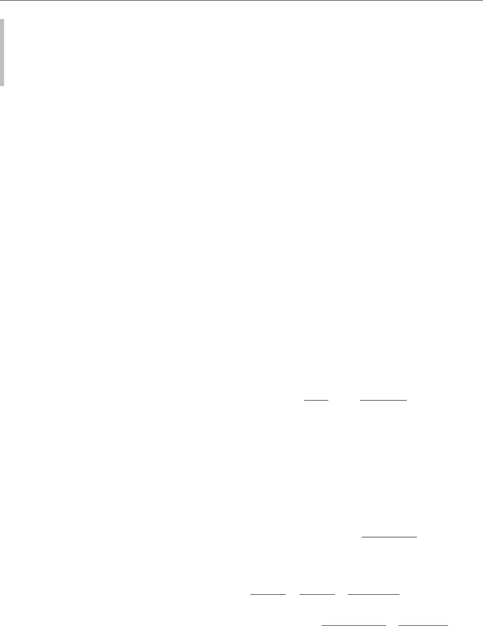
obtained by considering the graph elements shown in

Figure 1, where the segments will be called half-lines

and the graph elements will be called, respectively,

‘‘coupling’’ or ‘‘’

-vertex,’’ ‘‘mass vertex,’’ ‘‘vacuum

vertex,’’ and ‘‘external vertex.’’

The half-lines of the graph elements are consid-

ered distinct (i.e., imagine a label attached to

distinguish them). Then consider all possible con-

nected graphs G obtained by first drawing, respec-

tively, n, p, r graph elements in Figure 1, which are

not vacuum vertices, with their nodes marked by

points in  named x

, ..., x

, x

nþ1

, ..., x

nþpþr

; and

form all possible graphs obtained by attaching pairs

of half-lines emerging from the vertices of the graph

elements. These are the ‘‘nontrivial graphs.’’

Furthermore, consider also the single ‘‘trivial’’

graph form ed just by the third graph element and

consisting of a single point. All graphs obtained in

this way are particular Feynman graphs.

Given a nontrivial graph G (there are many of

them) we define its value to be the product

ðx

; ...; x

; x

nþ1

; ...; x

nþpþr

¼ð1Þ

nþpþr





nþpþj

n!p!r!

‘

ðNÞ

‘

½11

where the last product runs over all pairs ‘ = (x

‘

, h

‘

)

of half-lines of G that are joined and connect two

vertices labeled by points x

‘

, h

‘

: ‘‘call line of G’’ any

such pair. If the graph consists of the single vacuum

ξξξ

Figure 1 The graph elements to representing ’

(N)4



, ’

(N)2

a constant ’

(N)

Constructive Quantum Field Theory 619

vertex its value will be 

. The series for

(1=jj) log Z

(, f ) is then



jj

ðx

; ...; x

nþpþr

j¼1

½12

and the integral will be called the integrated graph

value.

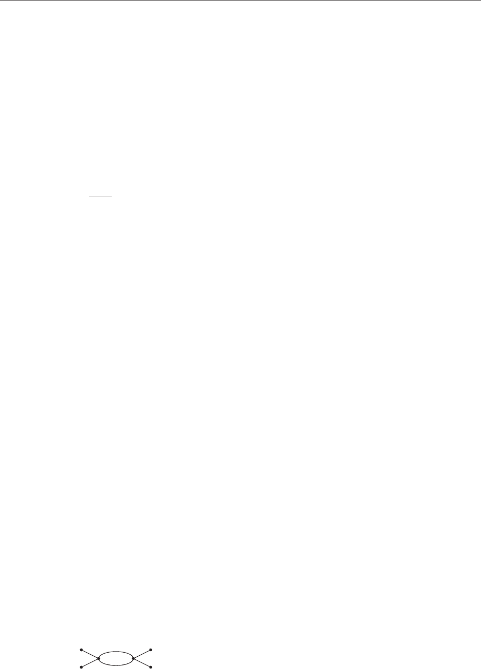
Suppose first that 

= 

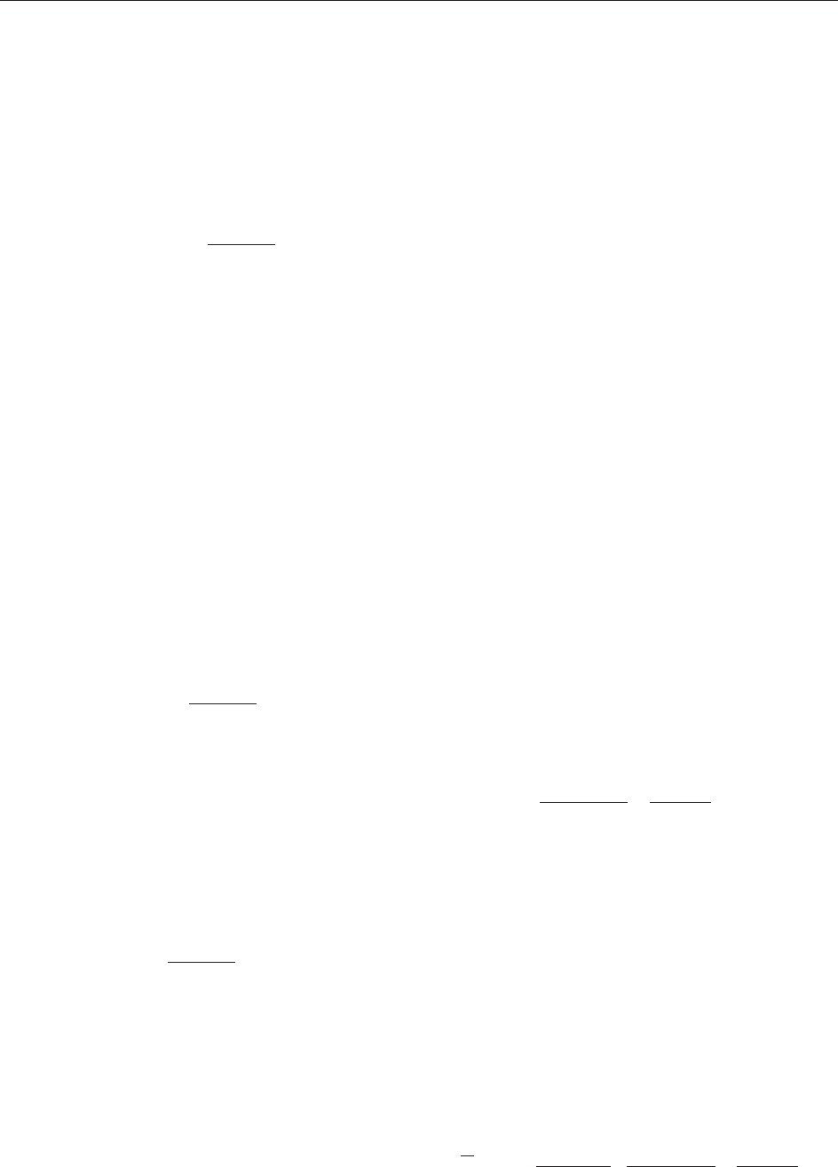
= 0. Then if a graph G

contains subgraphs like in Figure 2, the correspond-

ing respective contribution to the integral in [12]

(considering only the integrals over h and suitably

taking care of the combinatorial factors) is a factor

obtained by integrating over x the quantities

6C

ðN Þ

 3!



ðN Þ

ðN Þ3

ðNÞ

½13

which if d = 3 diverge as N !1 as 

or, respec-

tively, as N; the second factor does not diverge in

dimension d = 2 while the first still diverges as N. The

divergences arise from the fact that as x  h !0 the

propagator behaves as jx  hj

N

if d = 3oras

log jx  hj if d = 2, all the way until saturation

occurs at distance jx  hj’m

1



N

: for this reason

the latter divergences are called ‘‘ultraviolet

divergences.’’

However, if we set 

6¼ 0, then for e very gr aph

containing a subgraph like those in Figure 2 there

is another one identical except that the points

a, b are connected via a mass vertex, see Figure 1,

with the vertex in x, by a line ax and a line xb ;

the new graph value receives a contribution from

the mass vertex insert ed in x between a and b

simply given by a factor 

. T herefore if we fix,

for d = 3,



¼6C

ðN Þ

 3!







ðNÞ3

dh ¼

def

 6C

ðN Þ

þ 

½14

we can simply consider graphs which do not contain

any mass graph element and in which there are no

subgraphs like the first in Figure 2 while the subgraphs

like the second in Figure 2 do not contribute a factor

(N)

(N)3

(N)

dh but a renormalized factor

(N)

(N)3

(N)

 C

(N)

)dh.Ifd = 2, we only

need to define 

as the first term on the right-hand

side (RHS) of [14] and we can leave the subgraphs like

the second in Figure 2 as they are (without any

renormalization).

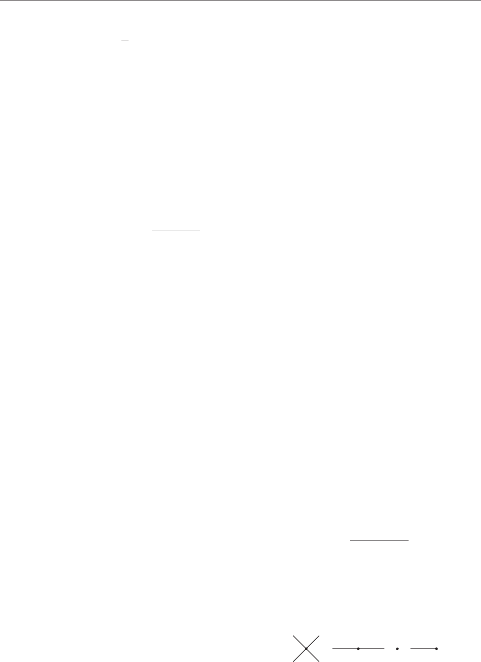
Graphs without external lines are called vacuum

graphs and there are a few such graphs which are

divergent. Namely, if d = 3, they are the first three

drawn in Figure 3; furthermore, if 

is set to the

above nonzero value a new vacuum graph, the

fourth in Figure 3, can be formed. Such graphs

contribute to the graph value, respectively, the terms

in the sum

3C

ðN Þ2



ðN Þ4



 3!





ðN Þ2

ðNÞ2

 

ðN Þ

½15

and diverge, respectively, as 

, 

, N, 

if d = 3

while, if d = 2, only the first and the last (see [14])

diverge, like N

Therefore, if we fix 

as minus the quanti ty in

[15] we can disregard graphs like those in Figure 3;

if d = 2 

can be defined to be the sum of the first

and last terms in [15].

The formal series in  and f thus obtained is called

the ‘‘renormalized series’’ for the field ’

dimension d = 2 or, respectively, d = 3. Note that

with the given definitions and choices of 

, 

the

only graphs G that need to be considered to

construct the expansion in  and f are formed by

the first and last graph elements in Figure 1, paying

attention that the graphs in Figure 3 do not

contribute and, if d = 3, the graphs with subgraphs

like the second in Figure 2 have to be computed with

the modification described.

In the next section, it will be shown that the

above are the only sources of divergences as N !1

and therefore the problem of studying [1] is solved

at the level of formal power series by the subtraction

in [14]. This also shows that giving a meaning to the

series thus obtained is likely to be much easier if

d = 2 than if d = 3.

The coefficie nts of order k of the expansion in 

of (1=jj) log Z

(, f ) can be ordered by the number

2n of vertices representing external fields : and have

the form

(k)

( x

, ..., x

)

i = 1

): the kernels

(k)

are the Schwinger functions of order 2n, see the

section ‘‘Euclide an quantum fields .’’

ξαβξ

αβ

Figure 2 Divergent subgraphs, if d = 3. If d = 2 only the first

diverges.

Figure 3 Divergent vacuum graphs.

620 Constructive Quantum Field Theory

Remark If d = 4, the regularization at cutoff N in

[2] is not sufficient as in the subtraction procedure

smoothness of the first derivatives of the field

’

(N)

is necessary, while the regularization [2] does

not even imply [6], that is, not even Ho¨ lder

continuity. A higher regularization (i.e., using a



like the square of the 

in [3]). Furthermore,

the subtractions discussed in the case d = 3 are not

sufficient to generate a formal power series and

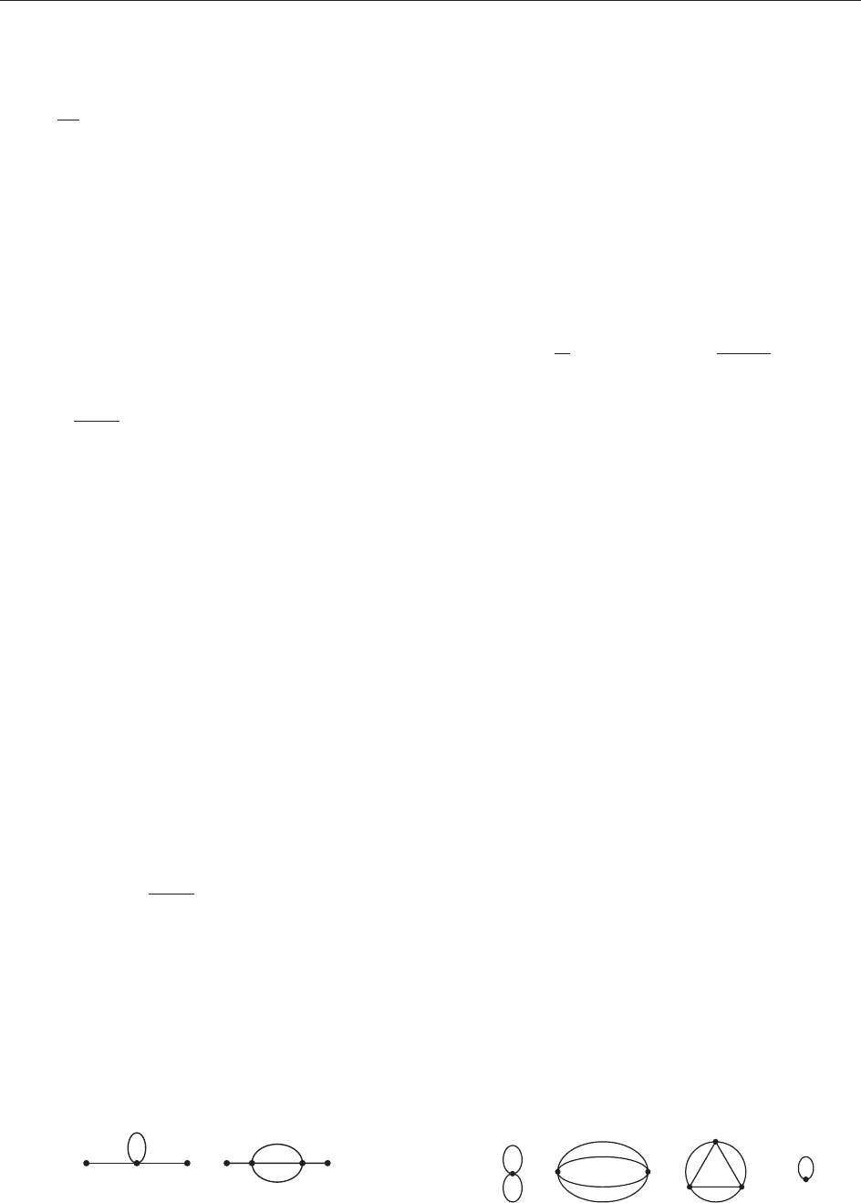
many more subtraction s are needed: for instance,

graphs with a subgraph like the one in Figure 4

would give a contribution to the graph value which

is a factor



‘

def

2  6



ðN Þ2

also divergent as N !1 proportionally to N.

Although this divergence could be canceled by

changing  into 

=  þ 

‘

the previously dis-

cussed cancelations would be affected and a change

in the value of 

would become necessary;

furthermore, the subtraction in [14] will not be

sufficient to make finite the graphs, not even to

second order in , unless a new term



’

(N)

)

dx with 

= (1=2)

(N)3

(x  h)

is added in the exponential in [1].

But all this will not be enough and still new

divergences, proportional to 

, will appear.

And so on indefinitely, the consequence being that

it will be necessary to define 

, 

, 

, 

formal power series in  (with coefficients diverging

as N !1) in order to obtain a formal power series

in  for [1] in which all coefficients have a finite

limit as N !1. Thus, the interpretation of the

formal renormalized series in the case d = 4is

substantially differe nt and naturally harder than

the cases d = 2, 3. Beyo nd formal perturbation

expansions, the case d = 4 is still an open problem:

the most widespread conjecture is that the series

cannot be given a meaning other than setting to 0 all

coefficients of 

, j > 0. In other words, the con-

jecture claims, there should be no nontrivial solution

to the ultraviolet problem for scalar ’

fields in

d = 4. But this is far from being proved, even at a

heuristic level. The situation is simpler if d  5: in

such cases, it is impossible to find formal power

series in  for (1=jj) log Z

(, f ), even allowing



, 

, 

, 

to be formal power series in  with

divergent coefficients.

The distinctions between the cases d = 2, 3, 4, >4

explain the terminology given to the ’

-scalar field

theories calling them super-renormalizable if

d = 2, 3, renormalizable if d = 4 and nonrenormaliz-

able if d > 4. Since the (divergent) coefficients in the

formal power series defining 

, 

, 

, 

are

called counter-terms , the ’

-scalar fields require

finitely many counter-terms (see [14]) in the super-

renormalizable cases and infinitely many in the

renormalizable case. The nonrenormalizable cases

(d > 4) cannot be treated in a way analogous to the

renormalizable ones.

For more details, the reader is referred

to Gallavotti (1985), Aizenman (1982),and

Fro¨ hli ch (1982).

Finiteness of the Renormalized Series,

d = 2, 3: ‘‘Power Counting’’

Checking that the renormalized series is well defined

to all orders is a simple dimensional estimate

characteristic of many multiscale arguments that in

physics have become familiar with the name of

‘‘renormalization group arguments.’’

Consider a graph G with n þ r vertices built over n

graph elements with vertices x

, ..., x

each with four

half-lines and r graph elements with vertices

nþ1

, ..., x

nþr

representing the external fields: as

remarked in the previous section, these are the only

graphs to be considered to form the renormalized series.

Develop each propagator into a sum of propaga-

tors as in [7]. The graph G value will, as a

consequence, be represented as a sum of values of

new graphs obtained from G by adding scale labels

on its lines and the value of the graph will

be computed as a product of factors in which a

line joining xh and bearing a scale label h

will contribute with C

(h)

replacing C

(N)

. To avoid

proliferation of symbols, we shall call the

graphs obtained in this way, i.e., with the scale

labels attached to each line, still G: no confusion

should arise as we shall, henceforth, only consider

graphs G with each line carrying also a scale label.

The scale labels added on the lines of the graph G

allow us to organize the vertices of G into

‘‘clusters’’: a cluster of scale h consists in a maximal

set of vertices (of the graph elements in the graph)

connected by lines of scale h

 h among which one

at least has scale h.

It is convenient to consider the vertices of the

graph elements as ‘‘trivial’’ clusters of highest scale:

conventionally call them clusters of scale N þ 1.

The clusters can be of ‘‘first generation’’ if they

contain only trivial clusters, of ‘‘second generation’’

Figure 4 The simplest new divergent subgraph on d = 4.

Constructive Quantum Field Theory 621

if they contain only clusters which are trivial or of

the first generation, and so on.

Imagine to enclose in a box the vert ices of graph

elements inside a cluster of the first generation and

then into a larger box the vertices of the clusters of

the second generation and so on: the set of boxes

ordered by inclusion can then be represented by a

rooted tree graph whose nodes correspond to the

clusters and whose ‘‘top points’’ are nodes represent-

ing the trivial clusters (i.e., the vertices of the graph).

If the maximum number of nodes that have to be

crossed to reach a top point of the tree starting from

a node v is n

(v included and the top nodes

included), then the node v represents a cluster of the

th generation. The first node before the root is a

cluster containing all vertices of G and the root of

the tree will not be considered a node and it can

conventionally bear the scale label 0: it represents

symbolically the value of the graph.

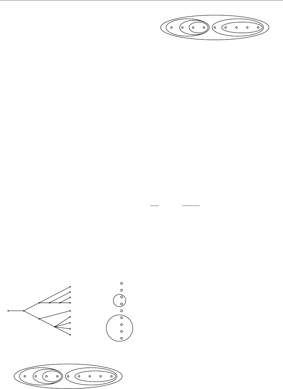
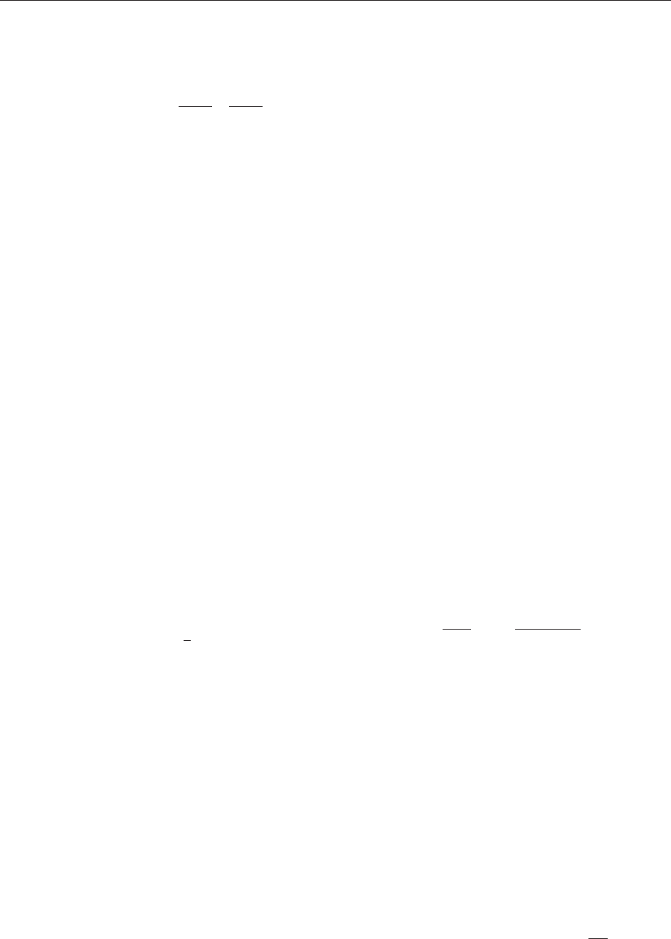
For instance, in Figure 5 a tree  is drawn: its

nodes correspond to clusters whose scale is indicated

next to them; in the second part of the drawing, the

trivial clusters as well as the clusters of the first

generation are enclosed into boxes.

Then consider the next genera tion clusters, that is,

the clusters which only contain clusters of the first

generation or trivial ones, and draw boxes enclosing

all the graph vertices that can be reached from each

of them by descending the tree, etc. Figure 6

represents all boxes (of any generation) correspond-

ing to the nodes of the tree in Figure 5. The

representations of the clusters of a graph G by a tree

or by hierarchically ordered boxes (see Figures 5 and

6) are completely equivalent provided inside each

box not representing a top point of the tree the scale

of the corresponding cluster v is marked. For

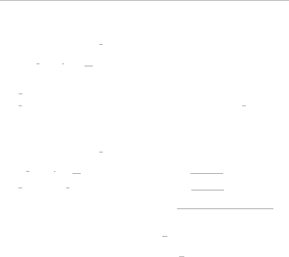
instance, in the case of Figure 6 one gets Figure 7.

By construction, if two top points x and h are inside

the same box b

of scale h

but not in inner boxe s,

then there is a path of graph lines joining x and h

all of which have scales h

and one at least has

scale h

Given a graph G, fix one of its points x

(say) and

integrate the absolute value of the graph over the

positions of the remaining points. The exponential

decay of the propagators implies that if a point h is

linked to a point h

by a line of scale h the

integration over the position of h

is essentially

constrained to extend only over a distance 

h

1

Furthermore, the maximum size of the propagator

associated with a line of scale h is bounded

proportionally to 

(d2)h

. Therefore, recalling that

j is suppose bounded by 1, the mentioned integral

can be immediately bounded by



n!r!

nþr

I ¼

def



nþr

n!r!

‘



ðd2Þ=2h

‘



dh

ðs

1Þ

½16

where, C being a suitable constant, the first product

is over the half-lines ‘ compos ing the graph lines and

the second is over the tree nodes (i.e., over the

clusters of the graph G), s

is the number of

subclusters contained in the cluster v but not in

inner clusters; and in [16] the scale of a half-line ‘ is

‘

if ‘ is paired with another half-line to form a line

‘ (in the graph G) of scale label h

‘

Denoting by v

the cluster immediately co ntaining

v in G,byn

inner

the number of half-lines in the

cluster v,byn

, r

the numbers of graph elements of

the first type or of the fourth type in Figure 1 with

vertices in the cluster v, and denoting by n

the

number of lines which are not in the cluster v but

have one extreme on a vertex in v (‘‘lines external to

v’’), the identities (k = 0)

v>root

ðh

 kÞðs

 1Þ



v>root

ðh

 h

Þðn

þ r

 1Þ

v>root

ðh

 kÞn

inner



v>root

ðh

 h

inner

with

inner

def

þ r

 n

½17

123456789

Figure 6 All clusters of any generation for the tree in Figure 5.

k = 0 h

leads to

Figure 5 A tree and its clusters of generation 1 and 2.

k = 0

123456789

Figure 7 The clusters in Figure 6 after affixing the scale labels.

622 Constructive Quantum Field Theory

hold, so that the estimate [16] can be elaborated into

I 

v>r





ðh

h



def

d þð4  dÞn

þ r

d þ 2

d  2

½18

where h

= k = 0ifv is the first nontrivial node (i.e.,

= ro ot), and an estimate of the integral of the

absolute value of the graphs G with given tree

structure but different scale labels is proportional to



}

I < 1 if (and only if) 

> 0, 8v.

But there may be clusters v with only two

external lines n

= 2 and two graph vertices inside:

for which 

= 0. However, this can happen only if

d = 3 and in only one case: namely if the graph G

contains a subgraph of the second type in Figure 2

and the three intermediate lines form a cluster v of

scale h

while the other two lines are external to it:

hence on scale h

> h

. In this case, one has to

remember that the subtraction in the previous section

has led to a modification of the contribution of such a

subgraph to the value of the graph (integrated over

the position labels of the vertices). As discussed in the

previous section, the change amounts to replacing the

propagator C

)

h, b

by C

)

h, b

 C

)

x, b

This improves, in [18], the estimate of the contribu-

tion of the line joining h to b from being proportional

(h

)

dh to being proportional to

(h

)

 C

(h

)

)dh; and this changes the con-

tribution of the line hb from 

(d2)h

m

jxhj

(

jx  hj)

1=2

dh because C

)

is regular on scale



h

1

,see[10] with " = 1= 2.

Since x, h are in a cluster of higher scale h

this

means that the estimate is improved by 

(1=2)(h

h

)

In terms of the final estimate, this means that 

[18] can be improved to



= 

þ 1=2 for the

clusters for which 

= 0. Hence, the integrated

value of the graph G (after taking also into account

the integration over the initially selected vertex x

trivially giving a further factor jj by translation

invariance), and summed over the possible scale

labels is bounded proportionally to jj

}

I < 1

once the estimate of I is improved as described.

Note that the graphs contributing to the perturbation

series for (1=j j)logZ

(, f ) to order 

are finitely

many because the number r of external vertices is r 

2n þ 2 (since graphs must be connected). Hence, the

perturbation series is finite to all orders in .

The above is the renormalizability proof of the

scalar ’

-fields in dimension d = 2, 3. The theory is

renormalizable even if d = 4 as mentione d in the

remark at the end of the previous section. The

analysis would be very similar to the above: it is just

a little more involved power-counting argument.

For more details, the reader is referred to Hepp

(1966), Gallavotti (1985), sections 8 and 16.

Asymptotic Freedom (d = 2, 3).

Heuristic Analysis

Finiteness to all orders of the perturbation expan-

sions is by no means sufficient to prove the existence

of the ultraviolet limit for Z

(, f ) or for (1=jj)

log Z

(, f ): and a priori it might not even be

necessary. For this purpose, the first step is to check

uniform (upper and lower) boundedness of Z

(, f )

as N !1.

The reason behind the validity of a bound

jjE



(, f )

 Z

(, f )  e

jjE

(, f )

with E



(, f ) cutoff

independent has been made very clear after the

introduction of the renormalization group met hods

in field theory. The approach studies the integral

(, f ), recursively, decomposing the field ’

(N)

into its regular components z

(h)

, see [7],and

integrating first over z

(N)

, then over z

(N1)

and so on.

The idea emerges naturally if the potential V

[1] and [4] is written in terms of the ‘‘normalized’’

variables X

(N)

def



N(d2)=2

’

(N)

,see[6];hereifd = 2

the factor 

(d2)=2N

is interpreted as N

1=2

The key remark is that as far as the integration

over the small-scale component z

(N)

is concerned the

field X

(N)

is a sum of two fields of size of order 1

(statistically),

ðNÞ

 z

ðNÞ



þ 

ðd2Þ=2

ðN 1 Þ

if d = 2 this becomes

ðNÞ



1=2

ðNÞ



ðN  1Þ

1=2

ðN1Þ

and it can be considered to be smooth on scale m

1



N

(also statistically). Hence, approximately constant

and of size of order O(1) on the small cubes  of

volume 

dN

d

of the pavement Q

introduced

before [7]; at the same time it can be considered to

take (statistically) independent values on different cubes

of Q

. This is suggested by the inequalities [8]–[10].

Therefore, it is natural to decompose the potential

,see[5], as a sum over the small cubes  of volume



dN

d

of the pavement Q

as (see [14] for the

definition of 

, 

), taking henceforth m = 1,

ðz

ðNÞ

Þ¼

def



2Q



Nd





2ðd2ÞN

ðNÞ4



þ 



ðd2ÞN

ðNÞ2

þ

þ f



ðd2Þ=2N

ðNÞ



jj

½19

Constructive Quantum Field Theory 623

where 

(d2)N

is interpreted as N if d = 2. Hence, if

d = 3itis

ðz

ðNÞ

def



2Q



N



X

ðNÞ4

þ 

ðNÞ2





þ f





ðNÞ



jj

½20

where



def

ð6c

þ 

N

N

Þ;



def

3c

þ 



N

þ 

N

2N

and c

, c

, b

, computable from [15] and [14],

admit a limit as N !1. While if d = 2itis

ðz

ðNÞ

def



2Q



2N



X

ðNÞ4

þ 

ðNÞ2





þ f



ðNÞ



jj

½21

where



def

6c

and 

= 3c

and c

, compu-

table from [13], admits a limit as N !1.

The fields z

(N)

and X

(N1)

can be considered

constant over boxes  2Q

: z

(N)

= s



, X

(N1)

= x



for x 2  and the s



can be considered statistically

independent on the scale of the lattice Q

Therefore, [20] and [21] show that integration over

(N)

in the integral defining Z

(, f ) is not too

different from the computation of a partition func-

tion of a lattice continuous spin model in which the

‘‘spins’’ are s



and, most important, interact extre-

mely weakly if N is large. In fact, the coupling

constants are of order of a power of jX

(N1)

j times

O(

N

)ifd = 3(O(N



2N

)ifd = 2), or of order

O(

N(dþ2)=2

max jf

j), no matter how large  and f.

This says that the smallest scale fields are

extremely weakly coupled. The fields X

(N1)

can be

regarded as external fields of size that will be called

N 1

, of order 1 or even allowed to grow with a

power of N,see[6]. Their presence in V

does not

affect the size of the couplings, as far as the analysis

of the integral over z

(N)

is concerned, because the

couplings remain exponentially small in N,see[20]

and [21], being at worst multiplied by a power of

N 1

, i.e., changed by a factor which is a power of N.

The smallness of the coupling at small scale is a

property called ‘‘asymptotic freedom.’’ Once fields

and coordinates are ‘‘correctly scaled,’’ the real size

of the coupling becomes manifest, that is, it is

extremely small and the addends in V

proportional

to the ‘‘counter-terms’’ 

, 

, which looked

divergent when the fields were not properly scaled,

are in fact of the same order or much smaller than

the main ’

-term.

Therefore, the integration over z

(N)

can be, heur-

istically, performed by techniques well established

in statistical mechanics (i.e., by straightforward

perturbation expansions): at least if the field

(N1)

is smooth and bounded, as prescribed

by [6], with B = B

N1

growing as a power of N.

In this case, denoting symbolically the integration

over z

(N)

by P or by h...i, it can be expected that it

should give

dPz

ðNÞ



e

j;N1

þRðj;NÞjj

½22

where V

j; N 1

is the Taylor expansion of

log

dP(z

(N)

) in powers of  (hence essentially

in the very small parameter 

(4d)N

) truncated at

order j, that is,

1;N1

¼½hV

i

1

2;N1

¼hV

iþ

ðhV

ihV

2

3;N1

iþ

ðhV

ihV

ðhV

ihV

ÞihV

ðhV

ihV



3

; ...

½23

where []

j

denotes truncation to order j in ,

and

R(j, N) is a remainder (depending on ’

(N1)

)

which can be expected to be estimated, for d = 2, 3, by

Rðj; NÞj  Rðj; NÞ

def

ð N



ð4dÞN

jþ1



½24

for suitable constants C

, that is, a remainder

estimated by the (j þ 1)th power of the coupling

times the number of boxes of scale N in . The

relations [22]–[24] result from a naive Taylor

expansion (in  of the log

dP(z

(N)

), taking into

account that, in V

as a function of z

(N)

, the z

(N)

’s

appear multiplied by quantities at most of size



4d

,by[20] and [21] if jX

(N1)

jB

N1

In a statistical mechanics model for a lattice spin

system, such a calculation of Z

would lead to a

mean-field equation of state once the remainder was

neglected.

The peculiarity of field theory is that a relation like

[22] and [24] has to be applied again to V

j; N1

perform the integration over z

(N1)

and define V

j; N2

and, then, again to V

j; N2

.... Therefore, it will be

essential to perform the integral in [22] to an order

(in ) high enough so that the bound R(j, N)canbe

624 Constructive Quantum Field Theory