Graef M. Introduction to conventional transmission electron microscopy

Подождите немного. Документ загружается.

298 Getting started

aperture

Imaging

lens

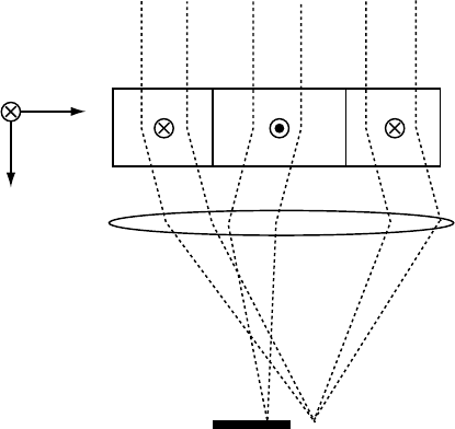
Fig. 4.30. Schematic illustration of the Foucault imaging mode.

know that the direction of the Lorentz deﬂection is normal to the corresponding

in-plane induction direction, we can use the four images in Fig. 4.31 to obtain a

schematic (qualitative) drawing of the magnetization conﬁguration, which is shown

in Fig. 4.28(b).

When more coherent illumination is used to obtain the Foucault images, fringes

are often observed parallel to the domain walls, inside the bright portions of the

image (e.g. [DDG97, Fig. 7]). The origin of these fringes is the same as for the

Fresnel mode and will be addressed in more detail in Section 7.5.2.

The Foucault mode is a highly qualitative observation mode, because it is no-

toriously difﬁcult to reproducibly position the aperture. Apertures are often not

perfectly circular, or may have debris at the aperture edge. When a set of four

Foucault images is acquired, it is difﬁcult if not impossible to manually (for me-

chanically controlled apertures) position the aperture at equal shifts from the central

beam position. This would be a prerequisite for quantitative work. It is also a non-

trivial task to determine the location of the optical axis, i.e. the position of the beam

in the absence of a magnetic sample. This position would be the “origin” for all

Foucault images, and one would have to specify the magnitude of the aperture shift

(typically in nm

−1

) with respect to this origin.

4.7.2.3 Diffraction mode

Figure 4.32(a) shows an electron diffraction pattern obtained from the divergent

part of a cross-tie wall in a 50 nm Permalloy thin ﬁlm. Since the saturation induction

4.7 Lorentz microscopy: observations on magnetic thin foils 299

-y +y

-x +x

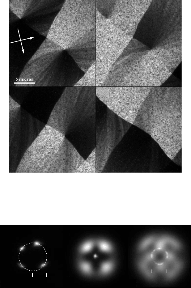
Fig. 4.31. Foucault images (zero-loss ﬁltered with 20 eV slit width, 400 kV) for four aperture

shifts for the same sample region as Fig. 4.28 (±x and ±y directions, with respect to the

aperture directions, indicated by the white arrows). The magnitude of the aperture shift is

approximately equal for all four images.

20µrad

40µrad

(a)

(b)

(c)

Fig. 4.32. (a) Electron diffraction pattern for the beam centered on the divergent part of

a cross-tie wall; each spot corresponds to the deﬂection from one of the quadrants of the

magnetization pattern. (b) Image of the undersaturated ﬁlament tip (LaB

), for the beam

passing through a single magnetic domain; (c) same as (b), but now the beam passes through

the convergent part (vortex) of a cross-tie wall.

300 Getting started

of this ﬁlm is about 1 T, the Lorentz deﬂection angle at 400 kV is about 20 µrad.

The pattern was acquired directly on the CCD camera of the energy ﬁlter, using

an under-saturated ﬁlament to prevent over-exposure of the camera. An exposure

time of 0.1 s was used, along with an energy selecting slit width of 20 eV. The

pattern is obtained by ﬁrst focusing the second condensor lens so that the gun

cross-over is conjugate to the specimen, and then adjusting the objective minilens

current to make the viewing screen (CCD plane) conjugate to the specimen. The

lateral magniﬁcation of the diffraction pattern can be adjusted by using the free-lens

control on the microscope, or the magniﬁcation reduction options on the energy

ﬁlter.

Figure 4.32(b) shows an image of the ﬁlament tip (LaB

) in an under-saturated

condition, when the beam passes through a single magnetic domain. The beam is

deﬂected from where it would be in the absence of a magnetic sample, but that

precise location is difﬁcult to determine experimentally. In Fig. 4.32(c) the incident

beam is focused on the vortex part of a cross-tie wall, and a nearly continuous

circular intensity distribution is obtained, along with a complex distribution from

the outer parts of the ﬁlament emission pattern. This pattern contains all the in-

formation about the momentum transfer due to the sample magnetization, but it

is complicated due to the fact that all magnetization directions around the vortex

contribute simultaneously to the image. If a ﬁne electron probe were scanned across

the region containing the cross-tie vortex, then a synchronized measurement of both

magnitude and direction of the deﬂection angle would provide a direct magnetiza-

tion map of the sample (actually, a map of the product B

⊥

t). This is essentially the

so-called differential phase contrast (DPC) acquisition mode [CBWF78].

4.8 Recommended additional reading

Before proceeding with the theory of dynamical elastic scattering, we conclude

this chapter with a brief list of additional reading material that the reader may

ﬁnd interesting. The following books (some of them are quite old and out-of-print

but you may ﬁnd them in your library) contain information on basic microscopy

techniques and sample preparation:

Transmission Electron Microscopy and Diffractometry of Materials, by B. Fultz and

J.M. Howe, 2001 [FH01].

Transmission Electron Microscopy, a Textbook for Materials Science, by D.B. Williams

and C.B. Carter, 1996 [WC96].

Transmission Electron Microscopy: Physics of Image Formation and Microanalysis,by

L. Reimer, 1993 [Rei93].

Specimen Preparation for Transmission Electron Microscopy of Materials, by P.J.

Goodhew, 1984 [Goo84].

Exercises 301

Electron Microscopy of Thin Crystals, by P.B. Hirsch, A. Howie, R.B. Nicholson,

D.W. Pashley, and M.J. Whelan, 1977 [HHN

77].

Practical Electron Microscopy in Materials Science, by J.W. Edington, 1976 [Edi76].

Computed Electron Micrographs and Defect Identiﬁcation, by A.K. Head, P. Humble,

L.M. Clarebrough, A.J. Morton, and C.T. Forwood, 1973 [HHC

73].

Introduction to Electron Microscopy, by C.E. Hall, 1953 [Hal53].

At this point we leave the experimental observations, and we set out to compute

and explain the details of the bright ﬁeld and dark ﬁeld images observed thus far.

This will require a fair number of mathematical calculations, but as a result we will

ﬁnd that many contrast features can be explained satisfactorily in terms of only a

small number of parameters.

Exercises

4.1 Ask one of your colleagues to intentionally misalign the microscope that you plan

to use. Then, carefully restore

the alignment to what it is supposed to be. Note that

you shouldn’t do this on a machine that is heavily used by more experienced users.

4.2 Derive the scaling factor needed to convert a length in the sample to a number of

pixels on a digital image of this sample. In other words, how many pix

els of the image

correspond to a given distance on the sample? You can use this relation to create a

table which expresses the number of pixels corresponding to different sample lengths

at all commonly used microscope magniﬁcations.

4.3 Compute the structure factor for Ti and verify that the reﬂections circled in

Fig. 4.18(b) are indeed forbidden reﬂections.

4.4 Perform a magniﬁcation and rotation calibration for the microscope that you plan

to work on for the foreseeable future. Estimate the accuracy of the magniﬁcation

calibration. Create a rotation chart similar to the one constructed in Fig. 4.17.

4.5 Perform a calibration of the camera lengths on the same microscope. Determine the

relative orientation of the diffraction pattern and corresponding image, including the

180

◦

ambiguity. Add this calibration data to the rotation chart that you constructed

in the previous exercise.

4.6 The relation between the distance measured on a diffraction pattern and the cor-

responding distance in

reciprocal space does not take into account the fact that

the Ewald sphere is curved. Derive a corrected expression and determine when the

corrections become important (e.g. when the corrections are larger than 5% of the

measured values).

4.7 Record a series of micrographs similar to that shown in Fig. 4.19. Use a small

selected area aperture to obtain systematic row diffraction patterns for different

aperture locations with respect to the bend contour

. Determine which portions of the

bend contour correspond to the so-called two-beam conditions (i.e. only two strongly

excited beams present in the systematic row).

302 Getting started

4.8 Use the

xtalinf

o.f90

program (or any equivalent program) to compute low-index zone

axis patterns for the study material Cu-15 at% Al. Then obtain a low-index zone

axis orientation in the microscope, write down the tilt angles, record both a bright

ﬁeld image and a diffraction pattern. Use either bend contours or Kikuchi lines (see

Section 9.4.3) to tilt to at least two other zone axis orientations for the same area of

the sample. Record diffraction patterns and write down the tilt angles. Then, after you

develop the negatives, index the zone axis patterns using the precomputed patterns,

and transfer the information to a stereographic projection. Determine the poles of the

100 family. Determine the direction indices of the foil normal (hint: if your foil is

not too strongly bent, you may assume that at zero tilt the incident beam is parallel

to the foil normal).

4.9 Record a zone axis diffraction pattern

for any one of the four study materials. Then tilt

the sample by 1

◦

around

the primary tilt axis and record the pattern. After you

develop the patterns, ﬁnd a way to calculate the tilt angle between the two patterns.

(Hint: use the position of the Laue center to ﬁnd an expression for the tilt angle.)

4.10 Obtain

111

systematic row CBED pattern for materials Cu-15 at% Al and GaAs.

Convince yourself that the symmetry of the g and −g disks is different for the non-

centrosymmetric structure, but identical for Cu-15 at% Al.

4.11 Use study material

Cu-15 at% Al, Ti, or BaTiO

to determine its average grain size

(use the calibrated magniﬁcation values). (You may wish to read about the ASTM

(American Society for Testing and Materials) standards for grain size measurements

[fTM98] before you start this exercise.)

Dynamical electron scattering in perfect crystals

5.1 Introduction

In the previous chapter, we have seen that electron micrographs can display a rich

variety of contrast features: thickness fringes, bend contours, intersections of bend

contours, defects, and so on. Now that we know the basic experimental techniques

to obtain the electron micrographs, we must take the next step and attempt to explain

all of these contrast features, for both images and electron diffraction patterns. We

have prepared the foundation for a theoretical description of electron scattering

through the derivation of the relevant Schr¨odinger equation in Chapter 2. Now

we must solve the equation for an arbitrary electrostatic lattice potential and an

arbitrary electron wavelength.

We know from the experiments in the preceding chapter that there are two basic

observation modes: two-beam observations, whereby only one diffracted beam has

appreciable intensity, and multi-beam observations, where the electron beam is

oriented close to a crystal zone axis, such that a plane in reciprocal space is nearly

tangent to the Ewald sphere. We will begin this series of theoretical chapters by ﬁrst

solving the equations for the most general case (i.e. the multi-beam case). Then we

will describe the two-beam case as a special case. While it is possible to approach the

elastic scattering problem in the opposite way, i.e. ﬁrst deal with the two-beam case

and then generalize the results to the multi-beam case, the method followed in this

and the next two chapters systematically deals with all important aspects of multi-

beam scattering, and the two-beam equations follow naturally from the results.

In this chapter, we will rephrase the governing equation (2.37) in several differ-

ent ways, and work out formal solution methods for the N -beam elastic scattering

problem. In Chapter 6, we simplify the results of this chapter and discuss the two-

beam case in great detail. Finally, in Chapter 7, we deal with the numerical solution

of the N -beam case for the systematic row and zone axis orientations. We will ﬁnd

that the methods described in these three theoretical chapters can be applied to a

303

304 Dynamical electron scattering in perfect crystals

large number of different experimental situations, among others: convergent beam

electron diffraction (CBED), high-resolution TEM, dynamical diffraction patterns,

Eades patterns, defect contrast analysis, and so on. While all three chapters rely

rather heavily on the mathematical formalism, the reader is encouraged to per-

sist and work through the equations. A good theoretical understanding of contrast

mechanisms will facilitate experimental work, since there is a direct relation be-

tween the mathematical formalism and what the microscope operator actually does

during a microscope session. Throughout the next three chapters, we will attempt

to highlight this relation whenever possible.

On the

website, the reader will ﬁnd a signiﬁcant amount of Fortran source code

dealing with the numerical solution of the N -beam elastic electron scattering prob-

lem. Some of this code is described in the text, but space restrictions do not permit

an extensive discussion of each routine or algorithm. The reader is encouraged once

more to study the source code and carry out some of the example runs suggested

on the

website. Most multi-beam simulations are too demanding computationally

to be performed in real-time, in particular through a website. Nevertheless, several

interactive ION routines are made available for limited real-time simulations. The

software will be discussed in Chapters 6 and 7. The theoretical

derivations in the

present chapter will be limited to formal solutions of the elastic scattering problem;

actual numerical solutions will be treated in Chapter 7.

In Section 5.8, we will analyze the intrinsic symmetry of the dynamical scattering

process, through the introduction of the reciprocity theorem and the diffraction

groups. We conclude this chapter with a brief historical review of the development

of the theory of elastic electron scattering.

5.2 The Schr¨odinger equation for dynamical electron scattering

The general equation for relativistic electron scattering is given by equation (2.37)

in Chapter 2:

 + 4π

 =−4π

U(r) =−

8π

(r). (5.1)

Note that we have replaced the electrostatic lattice potential V by the complex

potential V

= V + iW , introduced in Section 2.6.5. The Fourier transform of this

complex potential is given by

(r) = V

+ V



(r) + iW (r) = V



g=0

2πig·r

+ i



2πig·r

, (5.2)

where we have separated the zero-frequency component V

from the rest of the

Fourier series. V

is the positive mean inner potential, usually on the order of 5–50 V.

5.2 The Schr

odinger equation for dynamical electron scattering 305

Since it is positive, this potential accelerates the electrons when they enter the

crystal, and hence the relativistic acceleration potential of the electron increases to



 + γ V

. (5.3)

This acceleration is known as refraction, and is equivalent to the change of the

velocity of light when a photon enters a transparent medium with a refractive index

different from that of vacuum.

†

We deﬁne the wave number k

as follows:

≡



2me



. (5.4)

We introduce the following shorthand notation:

U (r) + iU



(r) ≡

2me



(r) + iW (r)].

In other words,

U(r) =

2me



g=0

2πig·r

;



(r) =

2me



2πig·r

Note that U



contains the term W

, whereas U does not have a zero-frequency

component. This will become important later on. Using equation (5.4) we obtain:

‡

 + 4π

 =−4π

[U + iU



], (5.5)

which is the starting equation for this chapter.

In the absence of a crystal potential other than the mean inner potential V

, and

ignoring absorption, we have U + iU



= 0. This is known as the empty crystal

approximation. The solution to the resulting homogeneous equation is given by



(r) = e

2πik

·r

, (5.6)

i.e. a plane wave, corrected for refraction, as is veriﬁed easily by substitution into

equation (5.5). In what follows we will choose the positive z-direction along the

electron propagation direction, i.e. k

=|k

. We will assume that the e

-axis lies

along the projection of one of the reciprocal lattice vectors, say g, onto the plane

normal to the optical axis. Mathematically, this is represented by

 (k

× g) × k

†

In the case of light, of course, the velocity decreases as light enters a medium with a refractive index larger than

unity. For electrons, the velocity increases upon entering the crystal.

‡

From here on we will no longer write the r dependence, except where confusion could arise.

306 Dynamical electron scattering in perfect crystals

Furthermore, we will assume that the crystal is planar, with parallel top and bot-

tom surfaces, and that it is defect-free. The bottom surface of the crystal, i.e. on

the opposite side of the electron source, will be known as the exit plane of the

crystal.

5.3 General derivation of the Darwin–Howie–Whelan equations

Bragg’s law (equation 2.41) tells us that electrons are diffracted in directions k



given by k

+ g, for all reciprocal lattice points g on the Ewald sphere. Hence,

we anticipate that the total wave function at the exit plane of the crystal will be a

superposition of plane waves, one in each of the directions predicted by the Bragg

equation. All that remains to be computed is the complex amplitude of each of these

diffracted waves. The general solution to equation (5.5) must then be of the form:

(r) =



2πi(k

+g)·r

. (5.7)

Note that this is a rather important assumption: instead of writing the total wave

function as a general superposition of momentum eigenfunctions, as we did in

Chapter 2, we limit the allowed momentum states to those satisfying the Bragg

equation. In Section 5.7, we will remove this assumption and compute the allowed

wave vectors inside the crystal, rather than imposing them from the beginning.

At this point in time we are not interested in what happens inside the crystal; we

are only interested in the behavior of the scattered waves far from the crystal.

The geometry for which all diffracted waves emanate from the back surface of

the crystal is commonly known as the Laue case; the other geometry, with scat-

tered waves on the same side of the crystal as the incident beam, is known as the

Bragg case.

After substitution of (r) above into equation (5.5) and some straightforward

computations, we ﬁnd:





ψ

+ i4π (k

+ g) ·∇ψ

+ 4π

− (k

+ g)



2πi(k

+g)·r

=−4π



[U + iU



]ψ

2πi(k

+g)·r

It can be shown [VD76] that the ﬁrst term (Laplacian derivative) in this equation is

negligible for high-energy electrons; this is the so-called high-energy approxima-

tion, or, equivalently, the forward scattering approximation. The argument for the

validity of this approximation involves the formal solution of the complete second-

order differential equation. Van Dyck [VD76] has shown that the high-energy ap-

proximation is a good approximation for crystal thicknesses up to a few hundred

5.3 General derivation of the Darwin–Howie–Whelan equations 307

nanometers, depending on the average atomic number of the crystal. First-order

correction terms

†

to the high-energy approximation can be found in [VD76].

For a perfect planar slab of material, the wave function component ψ

cannot

depend on the lateral coordinates x and y, so the gradient, ∇ψ

, contains only a

derivative with respect to z. Consequently, using the general deﬁnition of the dot

product (1.3), we can rewrite the second term as

+ g) ·∇ψ

=|k

+ g|cos α

dψ

with α the angle between the vectors e

and k

+ g. Often, cos α can be approxi-

mated by 1, since the diffraction angle for high energy electrons is of the order of

a few milliradians. Rearranging terms, we ﬁnd:





dψ

− i2π

− (k

+ g)

2|k

+ g|cos α



2πi(k

+g)·r



iπ

(U + iU



)

+ g|cos α

2πi(k

+g)·r

. (5.8)

At this point, we must remove the r dependence of the potential U + iU



, so that

the only r dependence remaining will be that of the plane waves. We introduce the

Fourier expansion:

U + iU







+ iU





2πiq·r

. (5.9)

Note that U

= 0, since V

was separated out earlier on. The right-hand side of

equation (5.8) can be rewritten as follows (we represent the left-hand side by LHS):

LHS = iπ





+ iU





+ g|cos α

2πi(k

+q+g)·r

Since q is an arbitrary reciprocal lattice vector, we can replace it by any other

reciprocal lattice vector, say q = g



− g. This results in

LHS = iπ









−g

+ iU



−g



+ g|cos α

2πi(k



)·r

Finally, since both g and g



are summation variables, we can interchange them

without changing the result of the summation:

LHS = iπ









g−g



+ iU



g−g





+ g



|cos α



2πi(k

+g)·r

†

The correction factor is proportional to the cube of the electron wavelength.