Griffiths D.F., Higham D.J. Numerical Methods for Ordinary Differential Equations: Initial Value Problems

Подождите немного. Документ загружается.

146 11. Adaptive Step Size Selection

have a certain accuracy—three correct decimal places or four correct signif-

icant ﬁgures, for example. This is not always possible, as the following example

illustrates.

Example 11.1

Using knowledge of the exact solution of the IVP

(t) = 2t, x(0) = 0,

show that it is not possible to choose the sequence of step sizes h

in Euler’s

method so that the solution is correct to precisely 0.01 at each step.

The method is given by

n+1

= x

+ 2h

n+1

= t

+ h

with x

= t

= 0. Thus, x

= 0, t

= h

, while the exact solution at this time

is x(t

) = h

. The GE x(t

) − x

is equal to 0.01 when h

= 0.01; that is,

= 0.1. For the second step,

= x

+ 2h

where t

= 0.1, so x

= 0.2h

while x(t

) = (0.1 + h

)

. The GE is

x(t

) − x

= 0.01 + h

and can equal 0.01 only if h

= 0. It is not possible to obtain a GE of 0.01 after

two steps unless the GE after one step is less than this amount.

Thus, in order to obtain a given accuracy at time t = t

, say, it may be neces-

sary in some problems to have much greater accuracy at earlier times; in others,

lower accuracy may b e suﬃcient. While it is possible to devise algorithms that

can cope with both scenarios (see, for instance, Eriksson et al. [19]), most cur-

rent software for solving ODEs is not based on controlling the GE. Rather, the

most common strategy is to require the user to specify a number tol, called the

tolerance, and the software is designed to adapt the step size so that the LTE

at each step does not exceed this value.

Our aim here is to present a brief

introduction to this type of adaptive step size selection. We shall address only

one step methods, in which case the calculations are based on the relationship

n+1

= H(t

p+1

+ O(h

p+2

) (11.2)

The situation is a little more intricate in practice, since software is typically

designed to use a relative error tolerance in addition to an absolute error tolerance—

see, for instance, the book by Shampine et al. [63, Section 1.4]. We shall limit ourse lves

to just one tolerance.

11. Adaptive Step Si ze Selection 147

(for some function H(t)) between the step size h

and the leading term in the

LTE of a pth-order method

for the step from t = t

to t = t

n+1

The calculations are organized along the following lines. Suppose that the

pairs (t

, x

), (t

, x

), . . . , (t

, x

) have already bee n computed for some value

of n ≥ 0 along with a provisional value h

new

for h

, the le ngth of the next time

step. There are four main stages in the calculation of the next step.

(a) Set h

= h

new

and calculate provisional values of x

n+1

and t

n+1

= t

+ h

(b) Estimate a numerical value

n+1

for the LTE T

n+1

at t = t

n+1

based on

data currently available. (How this is done is method-speciﬁc and will be

described presently.)

n+1

< tol we could have used a larger step size, while if

n+1

> tol the

step we have taken is unacceptable and it will have to be recalculated with

a smaller step size .

In both situations we ask: “Based on (11.2), what step size, h

new

, would

have given an LTE exactly equal to tol?” From step (b) we know that

n+1

≈ H(t

p+1

, while to achieve |T

n+1

| = tol in (11.2) we require

tol ≈ |H(t

)|h

p+1

new

; (11.3)

so, after eliminating H(t

), we take h

new

to be

new

= h



tol

n+1



1/(p+1)

. (11.4)

This is used in two ways in the next stage.

(d) If the estimated value of LTE obtained in stage (b) is too large

—|T

| >

tol—the current step is rejected. In this case we return to the previous

step—stage (a) on this list—with the value of h

new

given by (11.4) and

recalculate x

n+1

and t

n+1

Otherwise we pro ce ed to the next time step with the values of (t

n+1

, x

n+1

)

and h

new

This process is common to all the methods we will describe and its implemen-

tation requires a means of calculating an estimate

n+1

of the LTE (T

n+1

) and

a suitable initial step length (h

For instance, T

n+1

= L

x(t

) = C

p+2

p+1

(p+1)

) + O(h

p+2

) for a pth-order

LMM (see Equation (4.18)) so H(t) = C

p+1

(p+1)

(t). The corresponding expression

for two-stage RK methods is given at the end of Section 9.4, but, as we shall see, the

function H(t) for RK methods is estimated indirectly.

In practice a little leeway is given and a step is rejected if, for example,

n+1

| > 1.1tol.

148 11. Adaptive Step Size Selection

Equation (11.4) implies that h

new

∝ tol

1/(p+1)

and, since the GE is of

order p, it follows that GE ∝ tol

p/(p+1)

. For this reason we conduct numerical

experiments in pairs with tolerances that diﬀer by a ratio of 10

p+1

. The size of

computed time steps should then diﬀer by a factor of about 10 and experiments

with the smaller tolerance should require about 10 times as many steps to

integrate over the same interval. Also, the GE in the two experiments should

diﬀer by a factor of 10

, so the smaller tolerance should have p more correct

decimal digits than the larger tolerance. This is often made clearer graphically

by plotting the scaled GE, deﬁned by

scaled GE =

tol

p/(p+1)

as a function of time. The curves produced by the two experiments should lie

roughly on top of each other.

In the remainder of this chapter we will present a number of examples to

illustrate how methods of diﬀerent types may be constructed and, via numerical

examples, give some indication of how they perform.

11.1 Taylor Series Methods

These are the most straightforward methods for which to design step size se-

lection, since the leading term in the LTE may be expressed in terms of x(t)

and t by forming successive derivatives of the ODE.

The TS(p) method is given by (see equation (3.5))

n+1

= x

+ h

+ ··· +

(p)

. (11.5)

The LTE for the step from t = t

to t = t

n+1

is given by

n+1

(p+1)!

p+1

(p+1)

) + O(h

p+2

in which the leading term can be approximated by replacing x

(p+1)

) by

(p+1)

. Thus,

n+1

(p+1)!

p+1

(p+1)

, (11.6)

whose right-hand side is a computable quantity since it can be expressed in

terms of the previously computed quantities h

, t

, and x

by diﬀerentiating

the ODE p times. With (11.4) and (11.6) the step size update is given by

new



(p + 1)! tol

(p+1)



1/(p+1)

; (11.7)

11.1 Taylor Series Methods 149

so, if the current step is accepted, we progress with h

n+1

= h

new

. Otherwise

the step is recomputed with h

= h

new

It remains to choose a suitable value for the ﬁrst step length h

. This may

be done by setting |T

| = tol, from which we ﬁnd



(p + 1)! tol

(p+1)

)



1/(p+1)

. (11.8)

Example 11.2

Apply the TS(1) and TS(2) methods to solve the IVP (see Example 2.1)

(t) = (1 − 2t)x(t), t > 0

x(0) = 1



(11.9)

using adaptive step size selection.

The TS(1) method at the nth step is Euler’s method with a step size h

n+1

= x

+ h

, t

n+1

= t

+ h

, (11.10)

where x

= (1 −2t

. By diﬀerentiating the ODE (see Example 2.1) we ﬁnd

) =



(1 − 2t

)

− 2



x(t

)

and this may be approximated by replacing the exact solution x(t

) by the

numerical solution x

at t = t

to give



(1 − 2t

)

− 2



. (11.11)

The step size update is then given by (11.4) with p = 1; that is,

new

= h



2 tol



1/2

. (11.12)

Finally, since t

= 0 and x

= 1 we ﬁnd from (11.11) that x

= −1 and so

equation (11.8) gives h

√

2 tol.

The denominator in (11.12) vanishes when x

n+1

= 0, but this is easily accom-

mo dated since Equation (11.10) then implies that f

n+1

= 0 so that x

n+2

= x

n+1

= 0

at all subsequent steps.

A more signiﬁcant problem would occur at t

(1 +

√

2), since it would lead

to x

= 0. When t

is close to this value the leading term in in T

n+1

may well be

much smaller than the remainder and our estimate of the LTE is likely to be too

small. Should this lead to h

new

being too large the check carried out at the end of

each step would reject the step and it would be recomputed with a smaller step size.

If it should happen that x

= 0, division by zero is avoided in our experiments by

choosing h

n+1

= h

150 11. Adaptive Step Size Selection

TS(1) TS(2)

tol No. steps Max. error tol No. steps Max. error

−2

21 8.3 × 10

−2

11 2.3 × 10

−2

−4

207 8.4 × 10

−3

−5

101 1.8 × 10

−4

Table 11.1 Numerical results for TS(1) and TS(2) methods for solving the

IVP (11.9) in Example 11.2

The results of numerical experiments with tol = 10

−2

and 10

−4

are reported

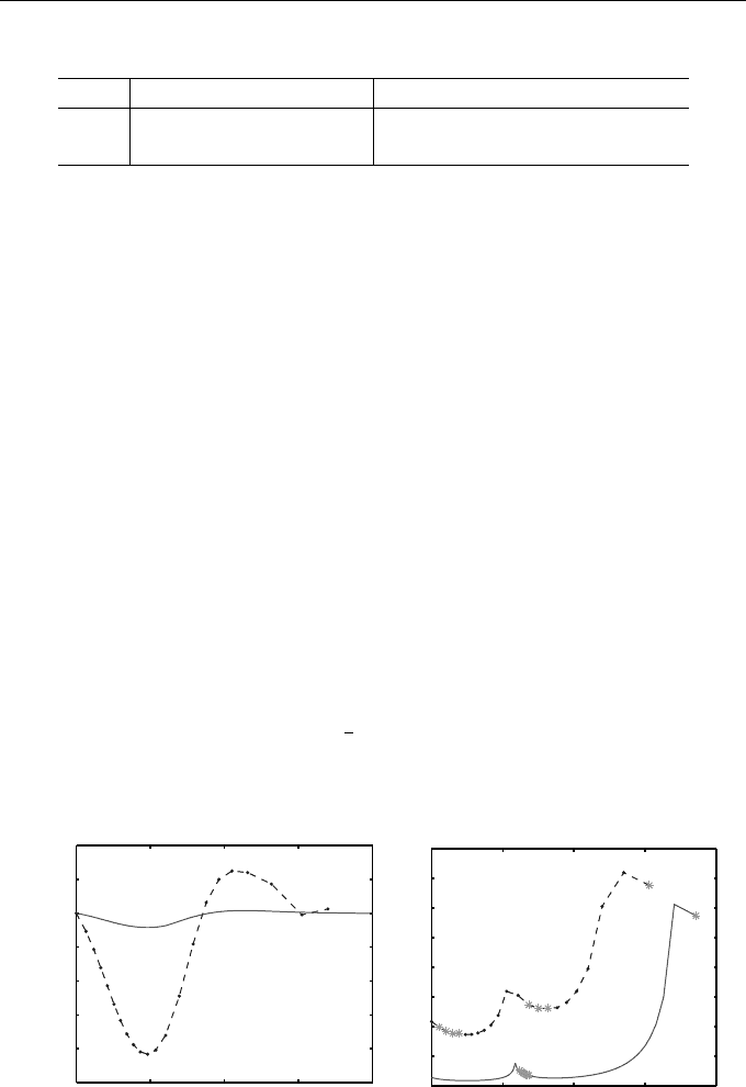
in Table 11.1 and Figure 11.1. The discussion on page 148, just before the start

of this section, suggests that h

new

∝ tol

1/2

; so, reducing tol by a factor of

100 should result in around 10 times as many time steps being required. This

is conﬁrmed by the second column of the table, where the number of steps

increases from 21 to 207. The results in the third column of the table show

that the GE is reduced (almost exactly) by a factor of 10 when tol is reduced

by a factor of 100, conﬁrming the expected relationship GE ∝ tol

1/2

In the time step history shown in Figure 11.1 (right) there is a local increase

in h

for t ≈ 1.2 corresponding to the zero in the denominator of (11.12) (see

footnote 5). It does not appear from the left-hand ﬁgure to have any signiﬁcant

eﬀect on the GE. The asterisks indicate rejected time steps (see stage (d) on

page 147). An explanation for the rejection of the ﬁnal step in each of the

simulations is oﬀered in Exercise 11.4.

For the second-order method TS(2) (see Example 3.1)

n+1

= x

+ h

, t

n+1

= t

+ h

, (11.13)

and the step size is updated using (11.7) with p = 2. The third derivative

0 1 2 3 4

−0.1

−0.08

−0.06

−0.04

−0.02

0.02

0.04

tol = 10

−2

tol = 10

−4

g e

0 1 2 3 4

0.05

0.1

0.15

0.2

0.25

0.3

0.35

0.4

tol = 10

−2

stepsize

tol = 10

−4

Fig. 11.1 Numerical res ults for Example 11.2 using TS(1). Shown are the

variation of GE (left) and time step h

(right) ve rsus time t

with tolerances

tol = 10

−2

, 10

−4

11.1 Taylor Series Methods 151

0 1 2 3 4

−0.1

0.1

0.2

0.3

0.4

0.5

0.6

tol = 10

−2

h = 1/3

g e

0 1 2 3 4

0.05

0.1

0.15

0.2

0.25

0.3

0.35

stepsize

tol = 10

−2

tol = 10

−5

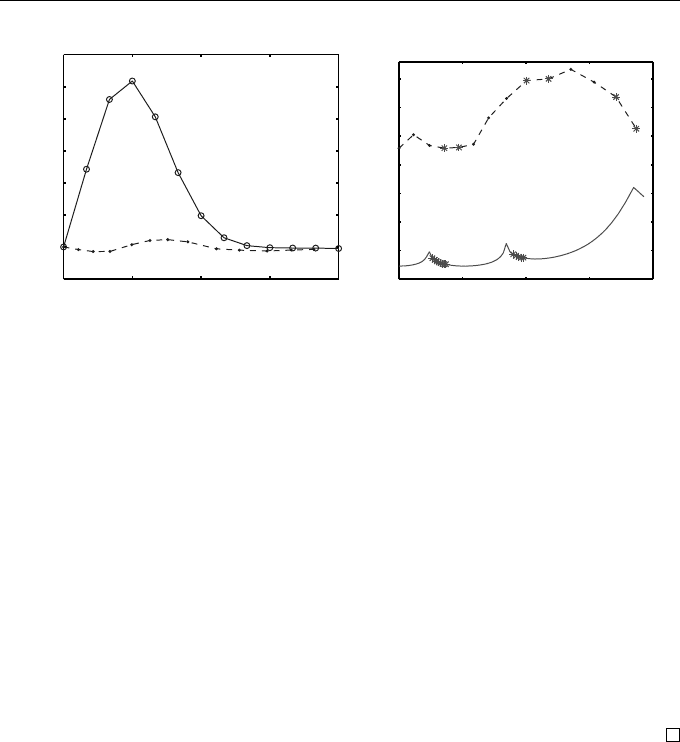
Fig. 11.2 Numerical results for Example 11.2 using TS(2). Left: the variation

of GE for the adaptive method with tol = 10

−2

(solid dots) and also the ﬁxed

time step method with h = 1/3 (circles). Right: time step h

versus time t

with tolerances tol = 10

−2

, 10

−5

. Asterisks (∗) indicate rejected steps

required can be found by diﬀerentiating the expression given earlier for x

(t).

The res ults of numerical experiments with tol = 10

−2

and 10

−5

shown in

Table 11.1 are in accordance with the estimates h

∝ tol

1/3

and GE ∝ tol

2/3

It is also evident that TS(2) achieves much greater accuracy than TS(1) with

substantially fewer steps.

The GE as a function of time is shown in Figure 11.2 (left) for tol = 10

−2

Also shown is the GE of the ﬁxed-step version of TS(2) described in Exam-

ple 3.2 that uses the same number of steps (12); thus, h = 1/3. The peak GE

of the ﬁxed-step method is more than 20 times larger than the variable-step

equivalent, illustrating the signiﬁcant gains in eﬃciency that can be achieve d

with the use of adaptive time steps.

Our ﬁnal example of the TS method illustrates how the same ideas can be

applied to the solution of systems of ODEs. It also serves as a warning that time

steps have to conform to the absolute stability requirements of the method.

Example 11.3

Use the TS(1) method with automatic time step selection to solve the IVP (1.14)

introduced in Example 1.9 to describe a cooling c up of coﬀee.

The system (1.14) can be written in the matrix-vector form x

(t) = Ax(t) + g,

where

x(t) =



u(t)

v(t)



, A =



−8 8

0 −1/8



, g =



5/8



and, since g is constant, x

(t) = Ax

(t) = A

x(t) + Ag. The initial condi-

152 11. Adaptive Step Size Selection

tion is x(0) = [100, 20]

. The equations in (11.10) have their obvious vector

counterparts:

n+1

= x

+ h

, t

n+1

= t

+ h

; (11.14)

to interpret the vector form of (11.12), we need a means of measuring the

magnitude of the vector x

. We shall use the Euclidean length, deﬁned by

kxk = (x

1/2

for a real vector x. Hence , (11.12) becomes

new

= h



2 tol



1/2

. (11.15)

The initial time step is given by the vector analogue of (11.8); that is,



2 tol



1/2

which gives h

≈ 0.0198×tol

1/2

. This, together with (11.14) and (11.15), serves

to deﬁne the method.

The numerical results obtained with this method for tol = 10

−2

and 10

−4

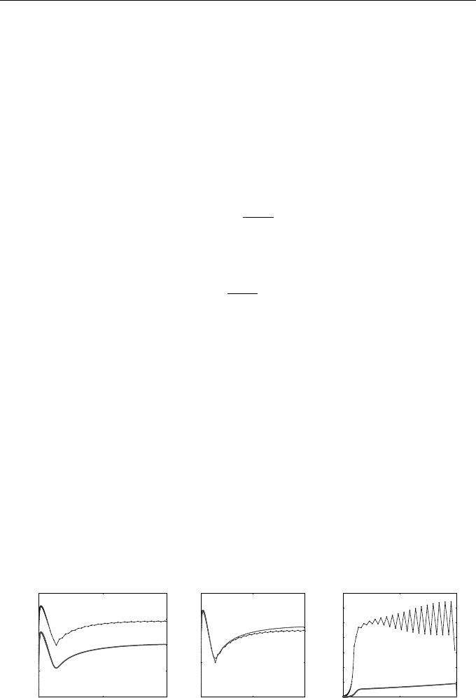
are shown in Figure 11.3. The GE shown on the left appears to behave as

expected—reducing tol by a factor of 100 reduces the GE by a factor of 10. To

check this more carefully we have plotted (middle) the GE scaled by tol

1/2

. The

two sets of results lie on top of each other for early times (up to about t = 2),

but there is evident divergence in the later stages, accompanied by perceptible

oscillations for tol = 10

−2

This departure from expected behaviour is due to the fairly violent oscilla-

tions in the time step, as se en in the rightmost plot. These, in turn, result from

the need to restrict the step sizes in order to achieve absolute stability (see

Chapter 6). To explain this, we ﬁrst note that the eigenvalues of the matrix

0 5 10

−4

−3

−2

−1

tol = 10

−2

tol = 10

−4

0 5 10

−2

−1

tol = 10

−2

tol = 10

−4

Scaled Error

0 5 10

0.05

0.1

0.15

0.2

0.25

0.3

tol = 10

−2

stepsize

tol = 10

−4

Fig. 11.3 Numerical res ults for Example 11.3 using TS(1). Shown are the

variation of GE (left), the scaled GE (that is, GE/tol

1/2

) (middle), and time

step h

(right) versus time t

. The tolerances used are tol = 10

−2

, 10

−4

11.2 One-Step Linear Multistep Methods 153

A—which govern the dynamics of the system—are λ = −8 and −1/8 and the

interval of absolute stability of Euler’s method (Example 6.7) is (−2, 0). It is

therefore necessary for

h ≡ λh ∈ (−2, 0) for each eigenvalue, that is, h ≤

Whenever formula (11.15) returns a value h

new

, instability causes an

increase in the local error. The step size is then reduced below this critical level

at the next step. The LTE is then smaller than tol, inducing an increase in step

size, and the oscillations therefore escalate with time.

Because the magnitude of the solution in this e xample is initially 100, com-

pared with 1 in previous examples, these tolerances are, relatively speaking,

100 times smaller than previously. Equivalent tolerances in this example would

need to be 100 times larger than those we have used, but these would have

led to even more severe oscillations in the time step. With tol = 10

−2

the level

of GE is roughly 0.1, which corresponds to a relative error of only 0.1%—so,

meeting the requirements of absolute stability leads to perhaps smaller GEs

than are strictly necessary for most applications.

The moral of this example is that methods with step size control can-

not overcome the requirements of absolute stability, and these requirements

may force smaller step sizes—and hence more computational eﬀort and higher

accuracy—than the choice of tol would suggest.

11.2 One-Step Linear Multistep Methods

The general procedure for selecting time steps for LMMs is essentially the same

as that for TS m ethods described in the previous section. The main diﬀerence

is that repeated diﬀerentiation of the diﬀerential equation cannot be used to

estimate the LTE, as this would negate the beneﬁts of using LMMs. Hence,

a new technique has to be devised for estimating higher derivatives x

000

), etc. of the exact solution.

The study of k-step LMMs with k > 1 becomes quite involved, so we will

restrict ourselves to the one-step case.

Example 11.4

Devise a strategy for selecting the step size in Euler’s me thod (TS(1)) that

does not require diﬀerentiation of the ODE. Illustrate by applying the method

to the IVP (11.9) used in Example 11.2.

The underlying method is the same as that in Example 11.2, namely

n+1

= x

+ h

, t

n+1

= t

+ h

154 11. Adaptive Step Size Selection

for which the LTE at the end of the current step is

n+1

) + O(h

The term x

n+1

) is approximated using the Taylor expansion of x

n+1

)

about the point t

n+1

) = x

) − h

) + O(h

which can be rearranged to give

) =

n+1

) − x

)

+ O(h

This can be estimated in terms of numerically computed quantities by

n+1

) ≈

n+1

− x

Hence, T

n+1

is approximated by

n+1

− x

), (11.16)

and this is used in (11.12)) to update the step size.

We choose a small initial

step size h

= 0.1tol and allow the adaptive mechanism to increase it automat-

ically during subsequent steps.

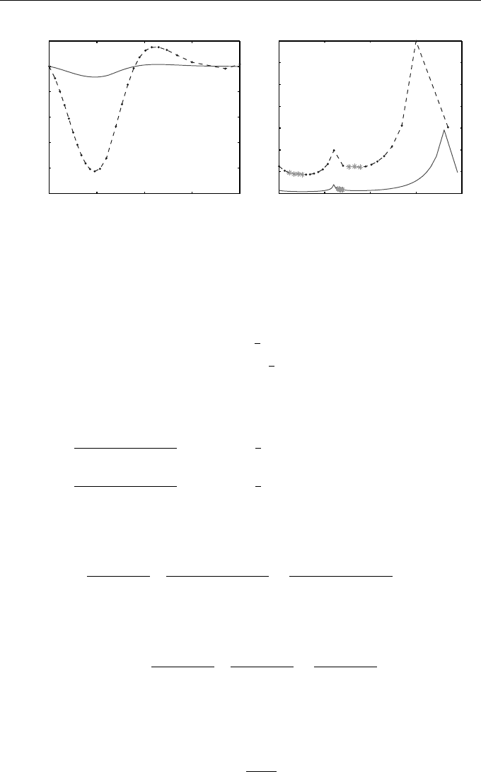
The results are shown in Figure 11.4 for tolerances tol = 10

−2

and 10

−4

It is not surprising that these show a strong resemblance to those for TS(1) in

Figure 11.1.

Example 11.5

Develop an algorithm based on the trapezoidal rule with automatic step size

selection and apply the result to the IVP of Example 11.2.

When h varies with n, the trapezoidal rule becomes

n+1

− x

n+1

+ f

) (11.17)

and the LTE at t = t

is given by (see Example 4.9)

n+1

= −

000

) + O(h

). (11.18)

The step-size-changing formula, (11.4) with p = 2, requires an estimate,

n+1

of T

n+1

. This will require us to estimate x

000

Notice that the values of x

and x

n+1

are already available, since they are re-

quired to apply Euler’s method. The cost of calculating

n+1

is therefore negligible.

11.2 One-Step Linear Multistep Methods 155

0 1 2 3 4

−0.1

−0.08

−0.06

−0.04

−0.02

0.02

tol = 10

−2

tol = 10

−4

g e

0 1 2 3 4

0.1

0.2

0.3

0.4

0.5

0.6

0.7

tol = 10

−2

stepsize

tol = 10

−4

Fig. 11.4 Numerical results for Example 11.4 using Euler’s method. Shown

are the variation of GE (left) and time step h

(right) versus time t

with

tolerances tol = 10

−2

, 10

−4

This is done by using the Taylor expansions (see Appendix B)

n+1

) = x

) + h

) +

000

) + O(h

n−1

) = x

) − h

n−1

) +

n−1

000

) + O(h

n−1

which make use of t

n+1

= t

+ h

and t

n−1

= t

− h

n−1

. When they are

rearranged as

n+1

) − x

)

= x

) +

000

) + O(h

) − x

n−1

)

n−1

= x

) −

n−1

000

) + O(h

n−1

) may b e eliminated by subtracting the second of these equations from

the ﬁrst. The resulting expression, when solved for x

000

), leads to

000

) =

+ h

n−1



n+1

) − x

)

−

) − x

n−1

)

n−1



+ O(h),

where we have used h to denote the larger of h

and h

n−1

in the remainder

term. Thus, x

000

) can be approximated by

000

) ≈

+ h

n−1



n+1

− x

−

− x

n−1



since it is written in terms of previously computed quantities x

n−1

, x

, and

n+1

. By combining these approximations we ﬁnd that the step size can be

updated via

new

= h



tol

n+1



1/3

, (11.19)