Griffiths D.F., Higham D.J. Numerical Methods for Ordinary Differential Equations: Initial Value Problems
Подождите немного. Документ загружается.


136 10. Runge-Kutta Methods–II Absolute Stability
b
h = λh, we find that
1
hk
1
= hf(t
n
, x
n
) = hλx
n
=
b
hx
n
,
hk
2
= hf(t
n
+ ah, x
n
+ ahk
1
),
=
b
h(x
n
+ ahk
1
) =
b
h(1 + a
b
h)x
n
.
Hence,
x
n+1
= x
n
+ (1 − θ)hk
1
+ θhk
2
=
1 +
b
h(1 + θa
b
h)
x
n
and, since aθ =
1
2
, it follows that
x
n+1
= R(
b
h)x
n
, (10.1)
where
R(
b
h) = 1 +
b
h +
1
2
b
h
2
(10.2)
is known as the stability function
2
of the RK method. Equation (10.1) is a
one-step difference equation having auxiliary equation (stability polynomial)
p(r) = r −
1 +
b
h +
1
2
b
h
2
.
Some remarks are in order:
(i) The stability function is linear in r and has only one root r = R (
b
h).
(ii) The stability function is the same for all explicit two-stage, second-order
RK methods—R(
b
h) does not depend on the parameter a.
(iii) The root r = R(
b
h) satisfies R(
b
h) = e
b
h
+O(
b
h
p+1
)) with p = 2 for this family
of second-order methods.
(iv) The solution of (10.1) will tend to zero as n → ∞, regardless of the value
of x
0
, if, and only if, |R(
b
h)| < 1; this is the c ondition for absolute stability.
The interval of absolute stability is the set of real values
b
h for which
|R(
b
h)| < 1. This leads to
−1 < 1 +
b
h +
1
2
b
h
2
< 1.
The left inequality is satisfied for all real
b
h and the right inequality is satisfied
if, and only if, −2 <
b
h < 0. This is the interval of stability. The boundary of the
1
It is usually more convenient to calculate hk
i
(for each i) since the result can be
expressed in terms of
b
h only, and does not involve h or λ separately.
2
Clearly, R (
b
h) is a polynomial in this example and is, indeed, a polynomial for all
explicit methods. However, as seen in Example 9.2, implicit methods lead to rational
expressions in
b
h.

10.1 Absolute Stability of RK Methods 137
region of absolute stability, despite having a rather a simple shape (Figure 10.1,
top right), is defined by a complicated expression (Exercise 10.9). What is
required is a means of computing the largest value of h for a given (complex)
value of λ. Writing λ = a + ib, then
b
h = h(a + ib) and it can be shown that the
equation |1 +
b
h +
1
2
b
h
2
|
2
= 1 leads to the following cubic polynomial in h:
(a
2
+ b
2
)
2
h
3
+ 4a(a
2
+ b
2
)h
2
+ 8a
2
h + 8a = 0. (10.3)
The real root of this equation gives the largest value of h for which the method
is absolutely stable.
10.1.1 s-Stage Methods of Order s
The results of Example 10.1 generalize to s-stage methods of order s (which
exist only for s ≤ 4—see Section 9.7) as follows:
(a) When applied to x
0
(t) = λx(t), the RK method leads to x
n+1
= R(
b
h)x
n
,
where the stability function R(
b
h) is a polynomial in
b
h of degree s (see
Exercises 10.7 and 10.8).
(b) Taylor expansion of the exact solution x(t
n+1
) about t = t
n
and using
x
0
(t) = λx(t), x
00
(t) = λ
2
x(t), etc., leads to
x(t
n+1
) =
1 +
b
h +
1
2!
b
h
2
+ ··· +
1
s!
b
h
s
x(t
n
) + O(
b
h
s+1
). (10.4)
(c) Under the localizing assumption x
n
= x(t
n
) and supposing the method to
have order s, then x
n+1
= x(t
n+1
) + O(h
s+1
). It follows from (a) and (b)
that
R(
b
h) = 1 +
b
h +
1
2!
b
h
2
+ ··· +
1
s!
b
h
s
. (10.5)
Thus, all s-stage, s-order RK methods have the same stability function,
R(
b
h). Clearly,
R(
b
h) = e
b
h
+ O(
b
h
s+1
).
Also |R(
b
h)| → ∞ as
b
h → −∞ so that no explicit RK method can be either
A-stable or A
0
-stable. The intervals/regions of absolute stability are defined as
the set of real/complex values of
b
h for which |R(
b
h)| < 1. (Since R(
b
h) = 1 at
b
h = 0, RK methods are always zero-stable.)
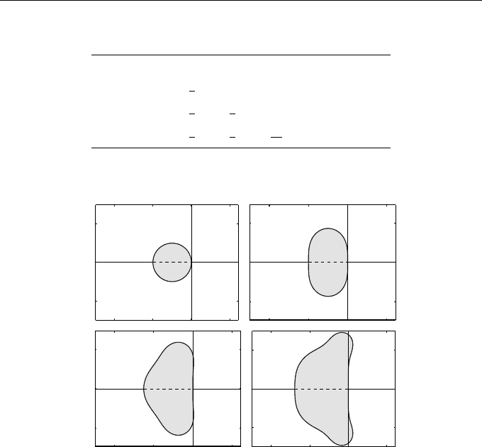
The intervals of absolute stability (IAS) of the four s-stage, sth-order RK
methods (1 ≤ s ≤ 4) are given in Table 10.1 and their regions of absolute
stability are shown in Figure 10.1. Note that the area of the region, as well as
the length of the interval of absolute stability, increases with s.
138 10. Runge-Kutta Methods–II Absolute Stability
s R(
b
h) IAS
1 1 +
b
h (−2, 0)
2 1 +
b
h +
1
2
b
h
2
(−2, 0)
3 1 +
b
h +
1
2
b
h
2
+
1
6
b
h
3
(−2.513, 0)
4 1 +
b
h +
1
2
b
h
2
+
1
6
b
h
3
+
1
24
b
h
4
(−2.785, 0)
Table 10.1 Intervals of absolute stability (IAS) for s-stage, s-order explicit
RK methods
−4 −2 0 2
−2
0
2
ℑ(λh )
ℜ(λh )
RK(1)
−4 −2 0 2
−2
0
2
ℑ(λh )
ℜ(λh )
RK(2)
−4 −2 0 2
−2
0
2
ℑ(λh )
ℜ(λh )
RK(3)
−4 −2 0 2
−2
0
2
ℑ(λh )
ℜ(λh )
RK(4)
Fig. 10.1 The region of of absolute stability for the s-stage, sth-order RK
methods. (RK(1) is Euler’s method: cf. Figure 6.6)
10.2 RK Methods for Systems
When applying explicit RK methods to IVPs for systems of the form
x
0
(t) = f (t, x(t)), t > t
0
x(t
0
) = η
, (10.6)
where x ∈ R
d
is a d-dimensional vector, each of the stage slopes k
1
, k
2
, . . . , k
s
becomes a vector. When performing hand calculations it may be preferable to
use a different symbol for each component of k
i
:
k
1
=
k
1
`
1
.
.
.
, k
2
=
k
2
`
2
.
.
.
, etc.
This is illustrated in the next example, which revisits Example 7.1.
10.2 RK Methods for Systems 139
Example 10.2
Use the improved Euler RK(2) method with h = 0.1 to determine the solution
at t = 0.1 of the IVP
u
0
(t) = −tu(t)v(t),
v
0
(t) = −u
2
(t),
with u = 1, v = 2 at t = 0.
The Butcher array of the improved Euler method is (Table 9.5 with θ =
1
2
)
0 0
1
2
1
2
0
1
2
1
2
n = 0 : t
0
= 0,
k
1
= −t
0
u
0
v
0
= 0,
`
1
= −u
2
0
= −1,
k
2
= −(t
0
+
1
2
h)(u
0
+
1
2
hk
1
)(v
0
+
1
2
h`
1
) = −0.0975,
`
2
= −(u
0
+
1
2
hk
1
)
2
= −1,
u
1
= u
0
+ h(k
1
+ k
2
) = 0.9902,
v
1
= v
0
+ h(`
1
+ `
2
) = 1.900,
t
1
= 0.1.
Note that u gets updated using k and the v gets updated using `. A possible
layout of calculations is shown in Table 10.2, where they are continued for one
further step.
n t
n
k
1
k
2
x
n
=
u
n
v
n
0 0.0 1
2 Initial data
1 0.1 0.0000 −0.0975 0.9902
−1.0000 −1.0000 1.9000
2 0.2 −0.1881 −0.2723 0.9630
−0.9806 −0.9621 1.8038
Table 10.2 Numerical solutions for the first two steps of Example 10.2

140 10. Runge-Kutta Methods–II Absolute Stability
10.3 Absolute Stability for Systems
The absolute stability of LMMs applied to systems was discussed in Sec-
tion 7.1—see Definition 7.4; a similar investigation is now carried out for RK
methods by applying them to the model problem
u
0
(t) = Au(t), (10.7)
where u(t) is an m-dimensional vector (u(t) ∈ R
m
) and A is a constant m ×m
matrix (A ∈ R
m×m
).
Example 10.3
Investigate the absolute stability properties of the family of second-order, two-
stage RK(2) methods.
The scalar version of this example is treated in Example 10.1. The correspond-
ing calculations are
hk
1
= hf (t
n
, u
n
) = hAu
n
,
hk
2
= hf (t
n
+ ah, u
n
+ ahk
1
)
= hA(u
n
+ ahk
1
) = hA(1 + ahA)u
n
.
Hence,
u
n+1
= u
n
+ (1 − θ)hk
1
+ θhk
2
=
1 + hA +
1
2
hA
2
u
n
(since aθ =
1
2
), so that
u
n+1
= R(hA)u
n
, (10.8)
where R(
b
h) is the stability function defined by equation (10.2). Thus, the
matrix-vector version is analogous to the scalar version provided that
b
h(= hλ)
is interpreted here as hA.
We assume, as in Section 7.1, that A is diagonalized by the matrix V , so
that V
−1
AV = Λ, where Λ is the diagonal matrix of eigenvalues. Then
V
−1
R(hA)V = R(hΛ)
(see Exercise 10.12). Multiplying both sides of (10.8) by V
−1
and applying the
change of variables u
n+j
= V x
n+j
leads to
x
n+1
= R(hΛ)x
n
,

10.3 Absolute Stability for Systems 141
a system in which all the components are uncoupled. If x
n
denotes a typical
component of x
n
and λ the corresponding eigenvalue, then
x
n+1
= R(
b
h)x
n
,
b
h = hλ,
the same equation that was obtained in the scalar case.
The results of this example generalize quite naturally to other explicit RK
methods; to ensure absolute stability,
b
h = hλ should lie in the region of absolute
stability of the method for every eigenvalue λ of A.
EXERCISES
10.1.
?
Verify that the two three-stage RK methods given in Table 9.7 have
the same stability function R(
b
h).
10.2.
??
Show, by considering the roots of the equations R(
b
h) = 1 and
R(
b
h) = −1, that all three-stage, third-order RK methods have the
same interval of absolute stability (h
∗
, 0), where h
∗
lies between −2
and −3.
10.3.
???
Apply the RK(4) method defined in Table 9.8 to the ODE x
0
(t) =
λx(t) and verify that it leads to x
n+1
= R(
b
h)x
n
, where R(
b
h) is
defined by (10.5) with s = 4.
Show that R(
b
h) may be written as
R(
b
h) =
1
4
+
1
3
(
b
h +
3
2
)
2
+
1
24
b
h
2
(
b
h + 2)
2
and deduce that the equation R(
b
h) = −1 has no real roots.
Prove that the method has interval of absolute stability (h
∗
, 0),
where R(h
∗
) = 1, and h
∗
lies between −2 and −3.
10.4.
??
Show that s-stage, sth-order RK methods have interval of stability
(h
∗
, 0) for s = 1, 2, 3, 4, where h
∗
is defined by R(h
∗
) = (−1)
s
.
10.5.
??
Use the Newton–Raphson method to solve the equations R(h
∗
) =
(−1)
s
for s = 3 and s = 4 obtained in the previous exercise. Use a
starting guess h
[0]
= −2.5 and verify that the roots agree with the
values given in Table 10.1 to three decimal places.
10.6.
??
Determine the interval of absolute stability for the RK method
k
1
= f(t
n
, x
n
),
k
2
= f(t
n
+ h/a, x
n
+ hk
1
/a),
x
n+1
= x
n
+ h((1 − a)k
1
+ ak
2
)

142 10. Runge-Kutta Methods–II Absolute Stability
and show that it is independent of the parameter a.
Show how the stability function for this method can be used to
establish an upper limit to its order of convergence.
10.7.
???
Supp ose that an RK method, defined by the Butcher array
c A
b
T
with c = (c
1
, . . . , c
s
)
T
, b = (b
1
, . . . , b
s
)
T
and A = (a
i,j
), an s × s
matrix, is applied to the scalar test equation x
0
(t) = λx(t). If k =
[k
1
, . . . , k
s
]
T
and e = [1, 1, . . . , 1]
T
, show that
k = λ(I −
b
hA)
−1
ex
n
.
Hence show that x
n+1
= R(
b
h)x
n
and the stability function R(
b
h) is
given by
R(
b
h) = 1 +
b
hb
T
(I −
b
hA)
−1
e.
10.8.
???
Using the Cayley–Hamilton Theorem, or otherwise, prove that
A
s
= 0 (it is nilpotent) when A is a strictly lower triangular s × s
matrix . Hence prove that
(I −
b
hA)
−1
= I +
b
hA +
b
h
2
A
2
+ ··· +
b
h
s−1
A
s−1
.
Deduce that, when A is the Butcher matrix for an explicit RK
method, the stability function R(
b
h) of Exercise 10.7 is a polynomial
in
b
h of degree s.
10.9.
???
The boundary of the region of absolute stability of all second-order
two-stage RK methods is given by |1 +
b
h +
1
2
b
h
2
| = 1. If
b
h = p + iq,
show that this leads to
(p + 1)
2
+
p
q
2
+ 1 − 1
2
= 1.
Hence, show that the boundary can be parameterized in real form
by
p = cos(φ) − 1, q = ±
p
(2 + sin(φ)) sin(φ)
for 0 ≤ φ ≤ π.
10.10.
?
If λ = −4 ± i show, using (10.3), that all two-stage, second-order
RK methods are absolutely stable for 0 < h < 0.498.
Exercises 143
10.11.
??
Show that any two-stage, second-order RK method applied to the
system u
0
(t) = Au(t), where
A =
−5 −2
2 −5
,
will be absolutely stable if h < 0.392. Hint: use (10.3).
What is the corresponding result for the matrix A =
−50 −20
20 −50
?
10.12.
??
Supp ose that the s × s matrix A is diagonalized by the s × s
matrix V :
V
−1
AV = Λ,
where Λ is an s ×s diagonal matrix. Prove that V also diagonalizes
all positive powers of A, i.e. V
−1
A
k
V = Λ
k
for any positive integer k.
Deduce that V
−1
R(hA)V = R(hΛ), where R(
b
h) is a polynomial of
degree s in
b
h.
10.13.
???
Prove that the method of Example 9.2 is A-stable, i.e. absolutely
stable for all <(
b
h) < 0.
[Hint: Write R(
b
h) = 1 +
b
h/D and show that |R(
b
h)|
2
− 1 < 0.]
10.14.
???
Show that the RK method given by the Butcher matrix
0 0
c c 0
c 1 − c
is consistent of order 1.
Show that one step of this method is equivalent to taking two steps
with Euler’s method—the first step with a step size ch and the sec-
ond with a step s ize (1 − c)h. When c =
1
2
(1 − γ), relate this to
the composite Euler method described in Exercise 6.21 and, hence,
deduce the interval of absolute stability of the given RK method.
10.15.
???
A semi-implicit RK method is given by the Butcher matrix
0 0 0 0
1
2
5
24
1
3
−
1
24
1 0 1 0
1
6
2
3
1
6
Determine the ratio x
n+1
/x
n
when the method is applied to x
0
(t) =
λx(t). Deduce that the method cannot be A-stable.

11
Adaptive Step Size S election
All the methods discuss ed thus far have been parameterized by the step size
h. The number of steps required to integrate over a given interval [0, t
f
] is
proportional to 1/h and the accuracy of the results is proportional to h
p
, for
a method of order p. Thus, halving h is expected to double
1
the amount of
computational effort while reducing the error by a factor of 2
p
(more than an
extra digit of accuracy if p > 3).
We now explore the possibility of taking a different step length, h
n
, at step
number n, say, in order to improve efficie ncy—to obtain the same accuracy with
fewer steps or better accuracy with the same number of steps. We want to adapt
the step size to local conditions—to take short steps when the solution varies
rapidly and longer steps when there is relatively little activity. The process
of calculating suitable s tep sizes should be automatic (by formula rather than
by human intervention) and inexpensive (accounting for a small percentage of
the overall computing cost, otherwise one might as well rep e at the calculations
with a smaller, constant step s ize h).
We shall describe methods for computing numerical solutions at times t =
t
0
, t
1
, t
2
, . . . that are not equally spaced, so we define the sequence of step sizes
h
n
= t
n+1
− t
n
, n = 0, 1, 2, . . . . (11.1)
What should be the strategy for calculating these step sizes? It appears in-
tuitively attractive that they be chosen so as to ensure that our solutions
1
These ball-park estimates are based on h being sufficiently small so that O(h
p
)
quantities are dominated by their leading terms.
Springer Undergraduate Mathematics Series, DOI 10.1007/978-0-85729-148-6_11,
© Springer-Verlag London Limited 2010
D.F. Griffiths, D.J. Higham, Numerical Methods for Ordinary Differential Equations,