Griffiths D.F., Higham D.J. Numerical Methods for Ordinary Differential Equations: Initial Value Problems
Подождите немного. Документ загружается.

156 11. Adaptive Step Size Selection
where (see equation (11.18))
b
T
n+1
= −
1
6
h
3
n
h
n
+ h
n−1
x
0
n+1
− x
0
n
h
n
−
x
0
n
− x
0
n−1
h
n−1
. (11.20)
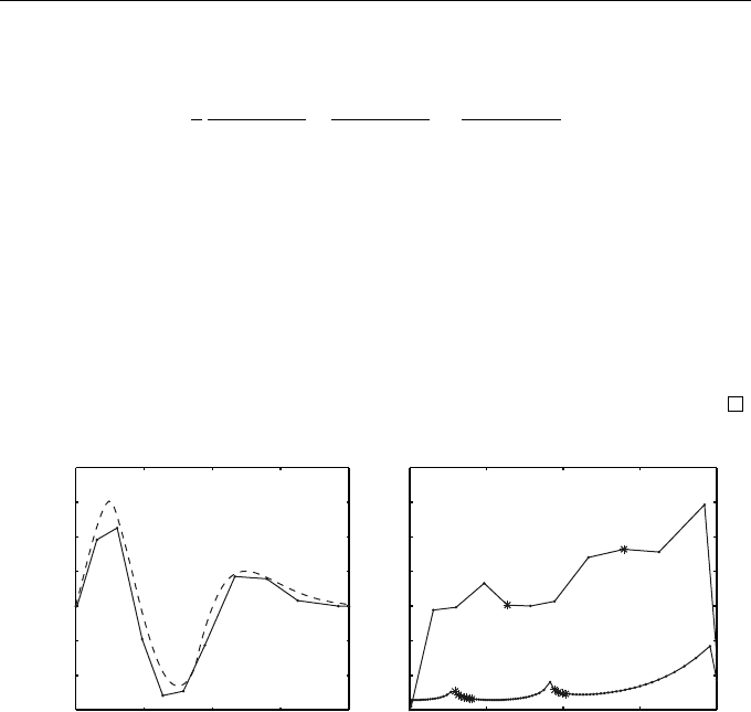
The integration process is initiated using two steps with very small time steps
(h
0
= h
1
= tol, say) and formula (11.19) is then used to predict a suitable step
size for subsequent time levels. We see in the right of Figure 11.5 that h
2
h
1
and the time steps immediately settle down to an appropriate level. Comparing
this figure with Figure 11.2 for TS(2) we see that the step sizes chosen for the
two methods are very similar.
For a second-order method the GE is expected to be proportional to tol
2/3
;
this is confirmed in the left part of Figure 11.5 where the scaled global errors
GE/tol
2/3
are approximately equal in the two cases.
0 1 2 3 4
−0.3
−0.2
−0.1
0
0.1
0.2
0.3
0.4
t
n
Scaled GE
0 1 2 3 4
0
0.1
0.2
0.3
0.4
0.5
0.6
0.7
t
n
h
n
tol = 10
−2
tol = 10
−5
Fig. 11.5 The numerical results for Example 11.5 using the trapezoidal rule.
Shown are the scaled GE (that is, GE/tol
2/3
) (left) and step sizes h
n
(right) ver-
sus t for tolerances tol = 10
−2
and 10
−5
(dashed curve). Asterisks (∗) indicate
rejected steps
11.3 Runge–Kutta Methods
We recall (Definition 9.3) that the LTE of an RK method is defined to be the
difference between the exact and the numerical solution of the IVP at time
t = t
n+1
under the localizing assumption that x
n
= x(t
n
); that is, the two
quantities were equal at the beginning of the step.
The idea here is to use two (related) RK methods, one of order p and another
of order p+1, to approximate the LTE. Suppose that these two methods produce
11.3 Runge–Kutta Methods 157
solutions x
hpi
n+1
and x
hp+1i
n+1
. Then the difference x
hp+1i
n+1
− x
hpi
n+1
will provide an
estimate of the error in the lower order method. Generally, such an approach
would be grossly inefficient, s ince it would involve computing two sets of k-
values. This duplication can be avoided by choosing the free parameters in our
methods so that the k values for the lower order method are a subset of those
of the higher order method (see Exercise 9.13). In this way we get two methods
almost for the price of one, and the LTE estimate can be obtained with little
additional computation.
Example 11.6 (RK(1,2))
Use Euler’s method together with the second-order improved Euler method
with Butcher tableau
0
1 1
1
2
1
2
to illustrate the construction of a method with adaptive step size control. Use
the resulting method to approximate the solution of the IVP of Example 11.2.
Since k
1
= f(t
n
, x
n
), we observe that x
n+1
= x
n
+ h
n
k
1
is simply the
one-stage, first-order method RK(1) (Euler’s method). Suppose we denote the
result of this calculation by x
h1i
; that is,
x
h1i
n+1
= x
n
+ h
n
k
1
. (11.21)
Also, if x
h2i
n+1
is the result of using the improved Euler method (see Section 9.4),
then
x
h2i
n+1
= x
n
+
1
2
h
n
k
1
+ k
2
, (11.22)
where k
2
= f
t
n
+h
n
, x
n
+h
n
k
1
. The LTE T
n+1
in Euler’s method at t = t
n+1
is estimated by the difference
b
T
n+1
= x
h2i
n+1
− x
h1i
n+1
,
so that the updating formula (11.4) gives
h
new
= h
n
tol
b
T
n+1
1/2
,
b
T
n+1
=
1
2
h
n
(k
2
− k
1
),
and we set x
n+1
= x
h1i
n+1
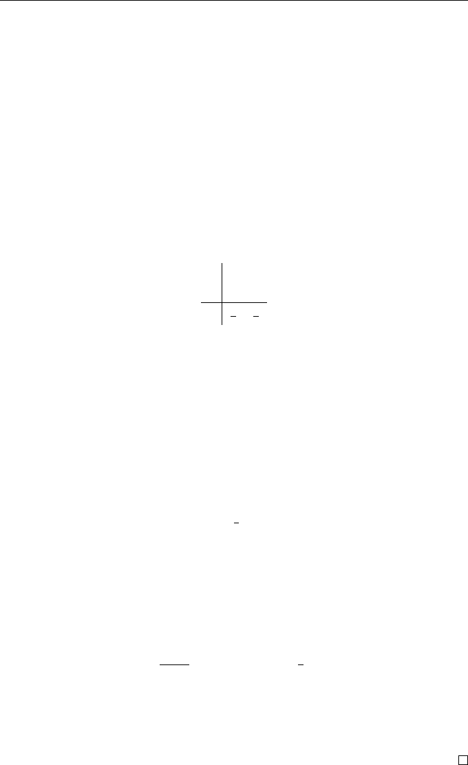
. When this method is applied to the IVP (11.9) with
h
0
= tol, the scaled GE and the time steps are shown in Figure 11.6 as functions
of time for tolerances tol = 10
−2
and 10
−4
. These show a strong similarity to
the results shown in Figures 11.1 and 11.4 for our other first-order methods.
158 11. Adaptive Step Size Selection
0 1 2 3 4
−1
−0.8
−0.6
−0.4
−0.2
0
0.2
0.4
t
n
Scaled g e
0 1 2 3 4
0
0.1
0.2
0.3
0.4
0.5
0.6
0.7
t
n
stepsize
tol = 10
−2
tol = 10
−4
Fig. 11.6 Numerical results for Example 11.2 using RK(1,2). The variation
of scaled GE (that is, GE/tol
1/2
) (left) and time step h
n
(right) versus time
t
n
with tolerances tol = 10
−2
(solid) and 10
−4
(dashed). Asterisks (∗) indicate
rejected steps
Example 11.7 (RK(2,3))
Use the third-order method with Butcher tableau
0 0
1 1 0
1
2
1
4
1
4
0
1
6
1
6
2
3
to illustrate the construction of a method with adaptive step size control. Use
the resulting method to approximate the solution of the IVP of Example 11.2.
When x
n+1
is computed using only the first two rows of this tableau
x
h2i
n+1
= x
n
+
1
2
h
n
k
1
+ k
2
we find that this metho d is the second order improved Euler method (see the
previous example). On the other hand,
x
h3i
n+1
= x
n
+
1
6
h
n
k
1
+ k
2
+ 4k
3
gives a method which is third-order accurate (see Exercise 11.14). The difference
x
h3i
n+1
− x
h2i
n+1
leads to the estimate
b
T
n+1
=
1
3
h
n
k
1
+ k
2
− 2k
3
11.4 Postscript 159
0 1 2 3 4
−0.4
−0.2
0
0.2
0.4
0.6
t
n
Scaled g e
0 1 2 3 4
0
0.05
0.1
0.15
0.2
0.25
0.3
0.35
0.4
t
n
stepsize
tol = 10
−2
tol = 10
−5
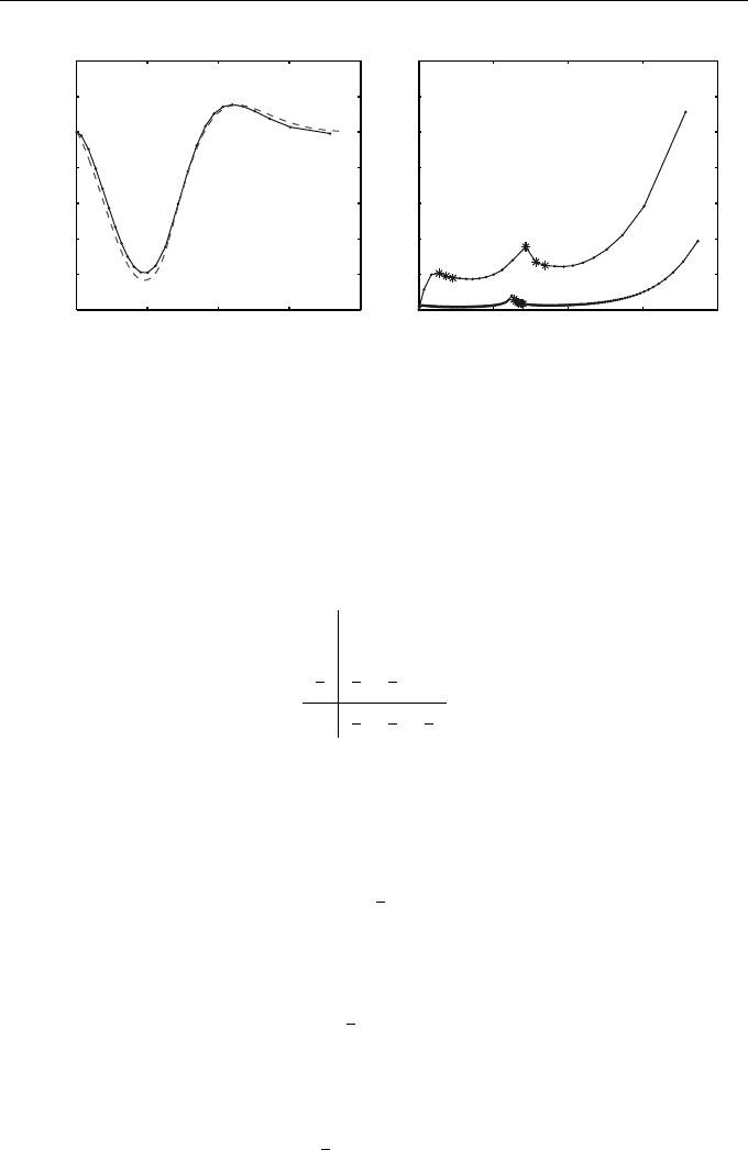
Fig. 11.7 Numerical results for Example 11.2 using RK(2,3). The variation
of scaled GE (that is, GE/tol
2/3
) (left) and time step h
n
(right) versus time
t
n
with tolerances tol = 10
−2
(solid) and 10
−5
(dashed). Asterisks (∗) indicate
rejected steps
for the LTE. Then, with p = 2 in (11.4), the update is given by
h
new
= h
n
tol
b
T
n+1
1/3
.
In our experiments we have used an initial step size h
0
= tol.
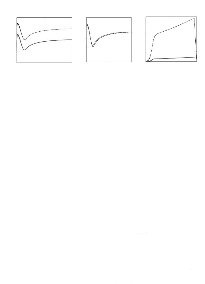
When applied to the the IVP of Example 11.2, the results are shown in
Figure 11.7. The correlation between the scaled GE with the two tolerances is
not as pronounced as with the other methods in this chapter (the correlation
improves as tol is reduced).
11.4 Postscript
A summary of the results obtained with the methods described in this chapter
is given in Table 11.2. The main points to observe are that:
(a) methods of the same order have very similar performance;
(b) second-order methods are much more efficient than first-order methods—
they deliver greater accuracy with fewer steps.
These conclusions apply only to nonstiff problems. On stiff systems the step
size will be restricted by absolute stability and, in these cases, implicit methods
would outperform explicit methods independently of their orders. For example,
when the IVP of Example 11.3 is solved by the backward Euler method (see

160 11. Adaptive Step Size Selection
tol = 10
−2
tol = 10
−4
No. steps Max. |GE| No. steps Max. |GE|
TS(1) 23(10) 0.081 209(8) 0.0084
Euler 25(7) 0.083 213(6) 0.0084
Backward Euler 24(5) 0.081 213(7) 0.0084
RK(1,2) 27(8) 0.079 216(9) 0.0083
tol = 10
−2
tol = 10
−5
TS(2) 12(7) 0.023 102(13) 0.00018
trapezoidal 13(2) 0.012 86(11) 0.00014
RK(2,3) 15(4) 0.027 98(11) 0.00015
RK(2,3)(Extrapolated) 14(4) 0.010 98(11) 0.00005
Table 11.2 Summary of numerical results for the methods described in this
chapter showing the number of steps to integrate over the interval (0, 4), the
number of rejected steps in parentheses, and the maximum |GE| taken over the
interval
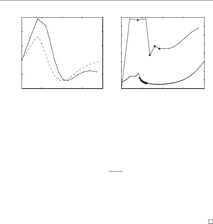
Exercise 11.8) rather than TS(1), we obtain the results shown in Figure 11.8.
On comparing Figures 11.3 and 11.8 we see that for the more relaxed tolerance
of 10
−2
the implicit method is allowed to use time steps that grow smoothly
with t because the error control strategy is not detecting any instability.
Rejected time steps impose an additional computational burden; in order
to reduce their occurrence, the main formula (11.4) for updating the step size
is often altered by including a “safety factor” of 0.9 on the right. The step size
used is therefore just 90% of the theoretically predicted value and will lead
to roughly 10% more steps being required—thus, this adjustment need only
be made if the number of rejected steps (which should be monitored as the
integration proceeds) approaches 10% of the number of steps used to date.
In RK methods the choice of step size is based on the estimate of the LTE
of the lower order method (x
hpi
). However, the solution x
hp+1i
would normally
be expected to give a more accurate approximation. It is common, therefore, to
use x
n+1
= x
hp+1i
n+1
when a step is accepted—the RK process is then said to be in
local extrapolation mode. The results for RK(2,3) operated in this way are shown
in the final row of Table 11.2 and, despite the lack of theoretical justification,
we see superior results to the basic RK(2,3) method. The codes for solving
IVPs presented in Matlab, for instance, use local extrapolation. Information
on these may be found in the book by Shampine et al. [63]. Moler [53] gives
a detailed description of the implementation of a simplified version of a (2,3)
Runge–Kutta pair devised by Bogacki and Shampine [4] that is the basis of the
Matlab function ode23.
Exercises 161
0 5 10
10
−4
10
−3
10
−2
10
−1
10
0
tol = 10
−2
tol = 10
−4
t
n
ge
0 5 10
10
−2
10
−1
10
0
10
1
tol = 10
−2
tol = 10
−4
t
n
Scaled Error
0 5 10
0
0.1
0.2
0.3
0.4
tol = 10
−2
t
n
stepsize
tol = 10
−4
Fig. 11.8 Numerical results for Example 11.3 using the backward Euler
method. Shown are the variation of GE (left), the scaled GE (that is, GE/tol
1/2
)
(middle), and time step h
n
(right) versus time t
n
. The tolerances used are
tol = 10
−2
, 10
−4
. These should be compared with the corresponding plots for
TS(1) shown in Figure 11.3
EXERCISES
11.1.
?
Show that the conclusion from Example 11.1 is true regardless of the
accuracy requested. That is , if h
0
is chosen so that |x(t
1
)−x
1
| = tol,
then |x(t
2
) − x
2
| = tol is unachievable for any choice of h
1
> 0.
11.2.
?
Repeat Example 11.1 for the backward Euler method
x
n+1
= x
n
+ 2h
n
t
n+1
, t
n+1
= t
n
+ h
n
.
(Note: in this case we require |x(t
n
) − x
n
| = 0.01 for each n.)
11.3.
?
Show that the TS(1) method described in Example 11.2 applied to
the IVP x
0
(t) = λx(t), x(0) = 1, leads to
x
n+1
= (1 + h
n
λ)x
n
, h
new
=
2 tol
λ
2
x
n
1/2
, x
0
= 1.
[This exercise is e xplored further in Exercise 13.12.]
11.4.
?
Prove for the TS(1) method described in Example 11.2 that|x
n+1
| <
|x
n
| (the analogue of absolute stability in this case) for t
n
>
1
2
if
h
n
<
2
2t
n
− 1
.
This implies that the step size must tend to zero as t → ∞ despite
the fact that the solution tends to zero. The final steps in the exper-
iments rep orted in Figure 11.1 (right) were rejected so as to avoid
h
n
exceeding this value. (This is a situation where using an implicit
LMM would be advantageous.)

162 11. Adaptive Step Size Selection
11.5.
??
Use a similar argument to that in the previous exercise to prove
that |x
n+1
| < |x
n
| for the TS(2) method described in Example 11.2
if
h
n
<
2(2t
n
− 1)
(2t
n
− 1)
2
− 2
when t
n
>
1
2
+
q
2
3
. Compare the limit imposed on h
n
by this in-
equality when t
n
≈ 3 with the two final rejected steps shown in
Figure 11.2 for tol = 10
−2
.
11.6.
?
Show that
x
000
(t) = (1 − 2t)
(1 − 2t)
2
− 6
x(t)
for the IVP (11.9). Use this in conjunction with Equation (11.7) for
p = 2 to explain the local maxima in the plot of h
n
versus t in
Figure 11.2 for t ≤ 2.
11.7.
??
Devise a step-sizing algorithm for TS(3) applied to the IVP (11.9).
11.8.
?
Explain why the step-size-changing formula for the backward Euler
method is identical to that for Euler’s method described in Exam-
ple 11.4.
11.9.
??
Show that the negative of the expression given by (11.16) provides
an estimate for the LTE of the backward Euler method. Show that
this estimate may also be derived via Milne’s device (8.11) for the
predictor-corrector pair described in Example 8.2.
11.10.
??
Calculate x
1
, t
1
, and h
1
when the IVP (11.9) is solved with h
0
= tol,
tol = 10
−2
, and (a) TS(1), (b) TS(2) and (c) Euler’s method (as in
Example 11.4).
11.11.
??
Calculate (t
1
, x
1
) and (t
2
, x
2
) when the IVP (11.9) is solved using
the trapezoidal rule with h
0
= h
1
= tol, tol = 10
−2
(see Exam-
ple 11.5).
11.12.
??
The coefficients of LMMs with step number k > 1 have to be
adjusted when the step sizes used are not the same for every step.
There is more than one way to do this, but for the AB(2) method
(Section 4.1.2) a popular choice is
x
n+1
= x
n
+
1
2
h
n
2 +
h
n
h
n−1
x
0
n
−
h
n
h
n−1
x
0
n−1
. (11.23)
The LTE of this method at t = t
n
is defined by
L
h
x(t
n
) = x(t
n+1
)−x(t
n
)−
1
2
h
n
2 +
h
n
h
n−1
x
0
(t
n
) −
h
n
h
n−1
x
0
(t
n−1
)
.
(11.24)

Exercises 163
Show, by Taylor expansion, that
L
h
x(t
n
) =
1
12
(2h
n
+ 3h
n−1
)h
2
n
x
000
(t
n
) + O(h
4
),
where h = max{h
n−1
, h
n
}.
11.13.
???
Supp ose that the Adams–Bashforth me thod AB(2) and the trape-
zoidal rule are to be used in predictor-corrector mode with variable
step sizes. Let x
[0]
n+1
and x
n+1
denote, respectively, the values com-
puted at t = t
n+1
by Equations (11.23) and (11.17). By following a
process similar to that described in Exercise 8.18 for constant step
sizes and using the expression for the LTE of the AB(2) method given
in the previous exercise, show that the generalization of Milne’s de-
vice (8.11) to this situation gives the estimate
b
T
n+1
= −
1
3
h
n
h
n
+ h
n−1
x
n+1
− x
[0]
n+1
for the LTE T
n+1
. Verify that this agrees with the estimate (11.20)
derived earlier in this chapter
7
. Verify that the result agrees with
that in Exercise 8.12 when h
n−1
= h
n
= h.
11.14.
?
Show, by using the results of Table 9.6, or otherwise, that the RK
method defined by the tableau in Example 11.7 is consistent of or-
der 3.
11.15.
???
Show that the modified Euler method (Table 9.5 with θ = 1) uses
two of the same k-values as Kutta’s third-order method (Table 9.7).
Write down an adaptive time-step process based on this pair of meth-
ods and verify, when it is applied to the IVP (11.9) with h
0
= tol
and tol = 0.01, that x
2
= 1.252 and t
2
= 0.321.
7
Writing the estimated LTE for the trapezoidal rule in terms of the difference
between predicted and corrected values is more common than using the form (11.20).

12
Long-Term Dynamics
There are many applications where one is concerned with the long-term be-
haviour of nonlinear ODEs. It is therefore of great interest to know whether
this behaviour is accurately captured when they are solved by numerical meth-
ods. We will restrict attention to autonomous systems of the form
1
x
0
(t) = f (x(t)) (12.1)
in which x ∈ R
m
and the function f depends only on x and not explicitly on t.
Equations of this type occur sufficiently often to make their study useful and
their analysis is much easier than for their non-autonomous counterparts where
f depends also on t. One immediate advantage is that we can work in the phase
plane. For example, if x = [x, y]
T
∈ R
2
, we may investigate the evolution of the
solution as a curve (x(t), y(t)) parameterized by t. See, for example, Figure 1.3
(right) for describing solutions of the Lotka–Volterra equations.
We will first discuss the behaviour of solutions of the differential equations—
the continuous case. This will be followed by an application of similar principles
to numerical methods applied to the differential equations—the discrete case.
The aim is to deduce qualitative information regarding solutions—building up
a picture of the behaviour of solutions without needing to find any general
solutions (which is rarely possible). The approach is to look for constant so-
lutions and then to investigate, by linearization, how nearby solutions behave.
1
Of course, as des cribed in Section 1.1, any non-autonomous ODE may be trans-
formed into autonomous form. However, this chapter focuses on autonomous ODEs
with fixed points, which rules out such a transformation.
Springer Undergraduate Mathematics Series, DOI 10.1007/978-0-85729-148-6_12,
© Springer-Verlag London Limited 2010
D.F. Griffiths, D.J. Higham, Numerical Methods for Ordinary Differential Equations,