Griffiths D.F., Higham D.J. Numerical Methods for Ordinary Differential Equations: Initial Value Problems

Подождите немного. Документ загружается.

166 12. Long-Term Dynamics

Our treatment will necessarily be brief; for further details we recommend the

bo oks by Braun [5, Chapter 4], Stuart and Humphries [65] and Verhulst [68].

12.1 The Continuous Case

Supp ose that x(t) = x

∗

, where x

∗

is a constant, is a solution of (12.1). Clearly

we must have f (x

∗

) = 0, and this motivates a deﬁnition.

Deﬁnition 12.1 (Fixed Point)

If x

∗

∈ R

satisﬁes f (x

∗

) = 0 then x

∗

is called a ﬁxed point

of the system

(12.1).

Supp ose that a solution becomes close to a ﬁxed point. Will this solution

be attracted towards it or be repelled away from it? The following deﬁnition

allows us to phrase this mathematically.

Deﬁnition 12.2 (Linear Stability)

A ﬁxed point x

∗

of (12.1) is linearly stable (or locally attracting) if there exists

a neighbourhood

around x

∗

such that any solution x(t) e ntering this neigh-

bourhood satisﬁes x(t) → x

∗

as t → ∞.

To investigate linear stability we write a solution of the ODE system in the

form

x(t) = x

∗

+ εu(t), (12.2)

where ε is a “small” real number, and ask whether u(t) grows or decays. We

do this by substituting (12.2) into (12.1) to obtain

εu

(t) = f (x

∗

+ εu(t)). (12.3)

Using the Taylor expansion of a function of several variables (see Appendix C)

f(x

∗

+ εu(t)) = f (x

∗

) + ε

∂f

∂x

∗

)u(t) + O(ε

)

Also known as an equilibrium point, critical point, rest state, or steady state.

The phrase “neighbourhood around x

∗

” means the set of points z within a sphere

of radius δ centred at x

∗

, for any positive value of δ. Thus, neighbourhoods can be

arbitrarily small but must contain x

∗

strictly in their interior.

12.1 The Continuous Case 167

and neglecting the O(ε

) term, (12.3) becomes, to ﬁrst order,

(t) = Au(t), (12.4)

where A is the m × m matrix

A =

∂f

∂x

∗

), (12.5)

known as the Jacobian of the system (12.1) at x

∗

. In two dimensions, where

x = [x, y]

∈ R

and f = [f, g]

, the matrix A has the 2 × 2 form

A =





The system (12.4) is known as the linearization of (12.1) at x

∗

, the idea being

that in the neighbourhood of x

∗

the behaviour of solutions of (12.1) can be

deduced by studying solutions of the linear system (12.4). From (12.2) we see

that u(t) shows us how a small perturbation from x

∗

evolves over time. A

suﬃcient condition that the s olution x = x

∗

be linearly stable is that u(t) → 0

in (12.4) as t → ∞. The next result follows from Theorem 7.3.

Theorem 12.3 (Linear Stability)

A ﬁxed point x

∗

of the system x

(t) = f (x(t)) is linearly stable if <(λ

) < 0

for every eigenvalue λ

of the Jacobian A =

∂f

∂x

∗

Example 12.4

Determine the ﬁxed points of the logistic equation x

(t) = 2x(t)



1 − x(t)



and

investigate whether they are linearly stable (see Example 2.2).

In this example we are dealing with scalar quantities (m = 1) with f(x) =

2x(1 − x). The ﬁxed points are given by f(x) = 0, and so x

∗

= 0 and x

∗

= 1.

The Jacobian is also scalar. It is given by the 1 × 1 matrix

∂f

∂x

(x) = 2 − 4x,

so that

∂f

∂x

(0) = 2 > 0 and

∂f

∂x

(1) = −2 < 0.

Hence, the ﬁxed point x

∗

= 0 is locally repelling—solutions starting close to

x = 0 will move further away—while x

∗

= 1 will attract nearby solutions. This

is illustrated in Figure 2.3, where a solution starting from x(0) = 0.2 moves

away from x = 0 and is attracted to x = 1 as t → ∞.

168 12. Long-Term Dynamics

Example 12.5

Investigate the nature of the ﬁxed points of the Lotka–Volterra system (see

Example 1.3

)

(t) = 0.05x(t)



1 − 0.01y(t)



(t) = 0.1y(t)



0.005x(t) − 2



(12.6)

Now

f(x) =



f(x, y)

g(x, y)



, f (x, y) = 0.05x(1 −0.01y), g(x, y) = 0.1y(0.005x −2).

The ﬁxed points are solutions of the simultaneous nonlinear algebraic equations

f(x, y) = 0 and g(x, y) = 0. These lead to the two ﬁxed points

∗





and x

∗



400

100



The Jacobian of the system is found to be

∂f

∂x

(x) =



0.05(1 − 0.01y) −0.0005x

0.0005y 0.1(0.005x − 2)



At the ﬁrst ﬁxed point x

∗

the Jacobian is

∂f

∂x

∗

) =



0.05 0

0 −0.2



whose eigenvalues are λ

= 0.05 and λ

= −0.2. One of these is positive, so

the origin is not an attracting ﬁxed point. At the s ec ond ﬁxed point x

∗

the

Jacobian is

∂f

∂x

∗

) =



0 −0.2

0.05 0



whose eigenvalues are λ

= ±0.1i. The real parts of both eigenvalues are zero,

so it is not possible to deduce the precise behaviour of the original system

without taking the nonlinear terms into account. This would take us beyond

the scope of this book (see Braun [5, Section 4.10] or Verhulst [68] for a detailed

study); we observe from Figure 1.3 that the motion is periodic (indicated by

the closed curves) around (400, 100), and this is in keeping with the ﬁndings

of Section 7.3, where imaginary eigenvalues were seen to be associated with

oscillatory behaviour.

We have used dependent variables x, y here so that u, v can be used for the

linearized system.

12.2 The Discrete Case 169

12.2 The Discrete Case

In this section we study the dynamical behaviour of the discrete map

n+1

= F (x

), (12.7)

where x

∈ R

and F (x) is assumed to be a continuously diﬀerentiable func-

tion of the m-dimensional vector x. In the context of numerical methods for

solving systems of ODEs such as (12.1), F is parameterized by the step size h:

Euler’s method, for example, leads to

F (x) = x + hf (x). (12.8)

Deﬁnition 12.6 (Fixed Point)

If x

∗

∈ R

satisﬁes x

∗

= F (x

∗

) then x

∗

is called a ﬁxed point of the discrete

map (12.7).

Deﬁnition 12.7 (Linear Stability)

A ﬁxed point x

∗

of (12.7) is linearly stable (or locally attracting) if there exists

a neighbourhood around x

∗

such that any solution x

entering this neighbour-

hoo d satisﬁes x

→ x

∗

as n → ∞.

Mimicking the continuous case, we can investigate linear stability by writing

= x

∗

+ εu

Substituting this into (12.7) and using the Taylor expansion

F (x

∗

+ εu

) = F (x

∗

) + ε

∂F

∂x

+ O(ε

)

we obtain, on neglecting terms of order O(ε

), the linearization of (12.7) at x

∗

n+1

= Bu

, (12.9)

where the m × m matrix

B =

∂F

∂x

∗

)

is the Jacobian of the function F (x) at x

∗

. The following is an analogue of

Theorem 12.3.

170 12. Long-Term Dynamics

Theorem 12.8 (Linear Stability)

A ﬁxed point x

∗

of the system x

n+1

= F (x

) is linearly stable if |λ

| < 1 for

every eigenvalue λ

of the Jacobian B =

∂F

∂x

∗

Proof

See, for example, Kelley [41, Theorem 1.3.2 and Chapter 4].

Some insight into Theorem 12.8 can be gleaned (using an argument similar to

that used in Section 8.2) by observing that if λ

is an e igenvalue of B with

corresponding eigenvector v then, choosing u

= v, the solution of (12.9) is

= λ

v. It follows that this u

cannot tend to zero as n → ∞ when |λ

| ≥ 1.

The next theorem gives an indication of the relationship between the ﬁxed

points of the ODE and those that result when the ODE is solved by Euler’s

method. Its conclusions remain true for all LMMs, but we will not prove this.

Theorem 12.9

Supp ose that Euler’s method is applied to the ODE system (12.1) leading to

the discrete map (12.7) with F (x) deﬁned in (12.8). Then x

∗

is a ﬁxed point

of (12.7) if, and only if, it is a ﬁxed point of (12.1).

Supp ose that x

∗

is a linearly stable ﬁxed point of (12.1) with <(λ

) < 0

for every eigenvalue λ

of the Jacobian A =

∂f

∂x

∗

). Then it is also a linearly

stable ﬁxed point of (12.7) provided that hλ

∈ R, the region of absolute

stability of Euler’s method (Figure 6.6), for every eigenvalue λ

of A.

Proof

The proof of the ﬁrst part is left as Exercise 12.2. For the second part, F (x) is

deﬁned by (12.8) so its Jacobian is given by

∂F

∂x

(x) = I + h

∂f

∂x

(x),

where I is the m × m identity matrix. Therefore, the matrix B in (12.9) is

related to the matrix A in (12.4) through

B = I + hA,

where I is the m ×m identity matrix, and it follows that the eigenvalues λ

A and λ

of B are related by (see Exercise 12.3)

= 1 + hλ

12.2 The Discrete Case 171

We are assuming that x

∗

is a linearly stable ﬁxed point of (12.1) and the

eigenvalues of A satisfy <(λ

) < 0. It follows from Theorem 12.8 that x

∗

will

also be a linearly stable ﬁxed point of Euler’s method provided |1 + hλ

| < 1,

which is the condition derived in Example 6.7 for

h = hλ

to lie in the region

of absolute stability.

We will show in Example 12.11 that the ﬁrst part of the previous theorem

is not true for the modiﬁed Euler method. In fact it does not hold for general

explicit RK methods, as they may admit ﬁxed points that are not ﬁxed points

of the ODE system.

Example 12.10

Investigate the linear stability of the ﬁxed points of the map obtained when

Euler’s method is applied to the ODE x

(t) = 2x(t)



1−x(t)



that was analysed

in Example 12.4.

The map is given by

n+1

= F (x

), where F (x) = x + hf(x), (12.10)

and f(x) = 2x(1 − x). It is readily shown that the ﬁxed points are x

∗

= 0, 1.

The Jacobian is the 1 × 1 matrix

∂F

∂x

(x) = 1 + 2h(1 − 2x)

and so

∂F

∂x

(0) = 1 + 2h and

∂F

∂x

(1) = 1 − 2h.

Since

∂F

∂x

(0) > 1 for all h > 0, the ﬁxed point x

∗

= 0 is not linearly stable and

all solutions close to x

= 0 are repelled.

At the other ﬁxed point x

∗

= 1 we have



∂F

∂x

(1)



= |1 − 2h| < 1

if, and only if, 0 < h < 1, in which case it is linearly stable.

In this example λ

= f

(1) = −2 and the interval of absolute stability of

Euler’s method is hλ

∈ (−2, 0). This translates to 0 < h < 1, conﬁrming the

relationship between linear stability of true ﬁxed points and absolute stability

of the numerical method identiﬁed in Theorem 12.9.

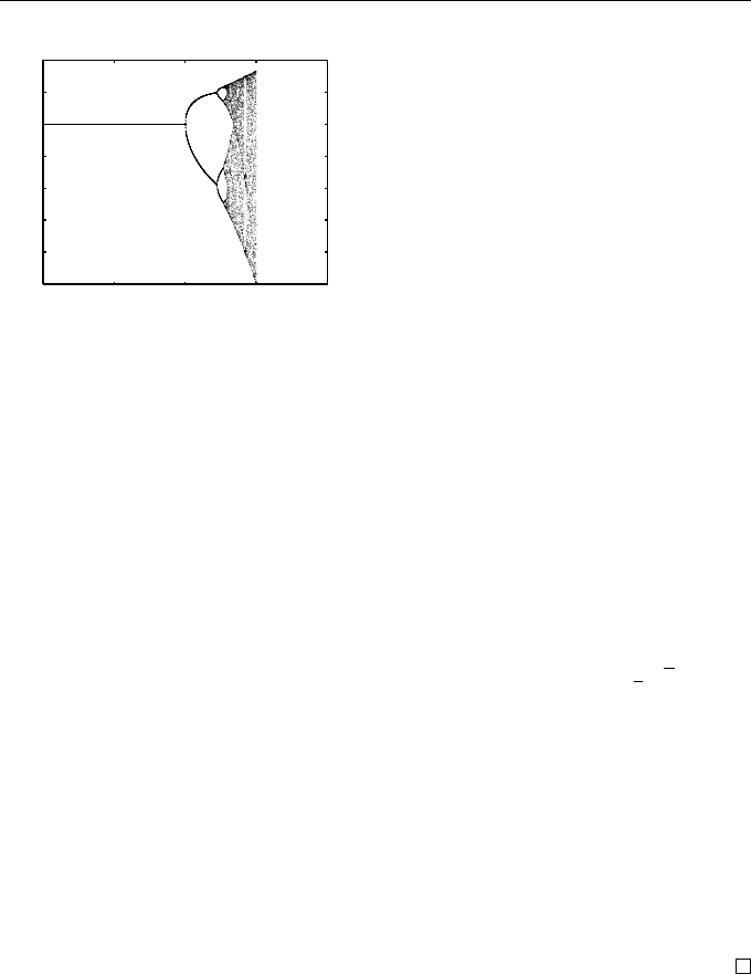
The results of an experiment to test these conclusions are shown in Fig-

ure 12.1. Here, we carried out the iteration (12.10) for 500 steps and then

plotted the p oints (h, x

) for the next 20 steps (where, if it possesses one, the

172 12. Long-Term Dynamics

0 0.5 1 1.5 2

0.2

0.4

0.6

0.8

1.2

1.4

Fig. 12.1 Bifurcation diagram for Eu-

ler’s m ethod applied to the logistic

equation of Example 12.4. The points

(h, x

), 500 < n ≤ 520 are plotted for

each h.

sequence would be expected to have reached its stable steady state to within

graphical accuracy). This process was repe ated for many values of h between

0 and 2 and several initial values were used for each value of h.

We see in Figure 12.1 that the sequence x

seems to settle down to the

ﬁxed point x

∗

= 1 for 0 < h < 1. The “ﬁxed point” branches to the right of

the value h = 1, x = 1—this is a “period 2” solution, where alternate values of

take the values a + b and a −b (see Exercise 12.4). This branching is known

as a bifurcation (literally to divide into two branches).

The period 2 solution can be found analytically by studying the ﬁxed points

of the iterated map x

n+1

= F(x

), where F(x) = F (F (x)), and its linear stabil-

ity analysed by calculating the Jacobian ∂F/∂x at the ﬁxed points. In this way,

it can be shown that the period 2 solution loses stability at h =

√

6 ≈ 1.22,

at which a further period-doubling occurs leading to a period 4 solution. Thes e

perio d-doublings continue along with other high-period solutions as h increases.

For certain values of h, the solution becomes “chaotic”—deﬁned loosely as a

sequence that does not repeat itself as n → ∞.

The bifurcation to a period 2 solution occurs when h increases so that hλ

leaves the region of absolute stability. This behaviour contrasts with that when

absolute s tability is lost in linear systems, where |x

| → ∞ as n → ∞ (see, for

example, Figure 6.2).

For detailed studies of similar quadratic maps see Thompson and Stew-

art [66, Section 9.2].

Our next example contains features common to many RK methods but not

present in the previous example.

Example 12.11

Determine the ﬁxed points of the modiﬁed Euler method described in Exam-

ple 9.1 when applied to the scalar equation x

(t) = 2x(t)



1−x(t)



and examine

their linear stability.

12.2 The Discrete Case 173

The method is deﬁned by the recurrence

n+1

= x

+ hf



hf(x

)



where f (x) = 2x(1 −x). To ﬁnd the ﬁxed points we set x

n+1

= x

= x so that

they satisfy the equation



x +

hf(x)



= 0.

Since f(y) = 0 has the two roots y = 0, 1, the ﬁxed points satisfy

x +

hf(x) = 0 or 1. (12.11)

These equations then lead to the four ﬁxed points (see Exercise 12.5)

∗

= 0, x

∗

= 1, x

∗

= 1/h, and x

∗

= 1 + 1/h. (12.12)

With F (x) = x + hf(x +

hf(x)) the Jacobian is given by

(x) = 1 + hf

(x +

hf(x))



1 +

(x)



(12.13)

with which it may be veriﬁed that

1. x

∗

= 0 is not linearly stable for any h > 0;

2. x

∗

= 1 is linearly stable for 0 < h < 1;

3. x

∗

= 1/h is linearly stable for 1 < h <

(1 +

√

5) ≈ 1.62;

4. x

∗

= 1 + 1/h is linearly stable for 1 < h <

(−1 +

√

5) ≈ 0.62.

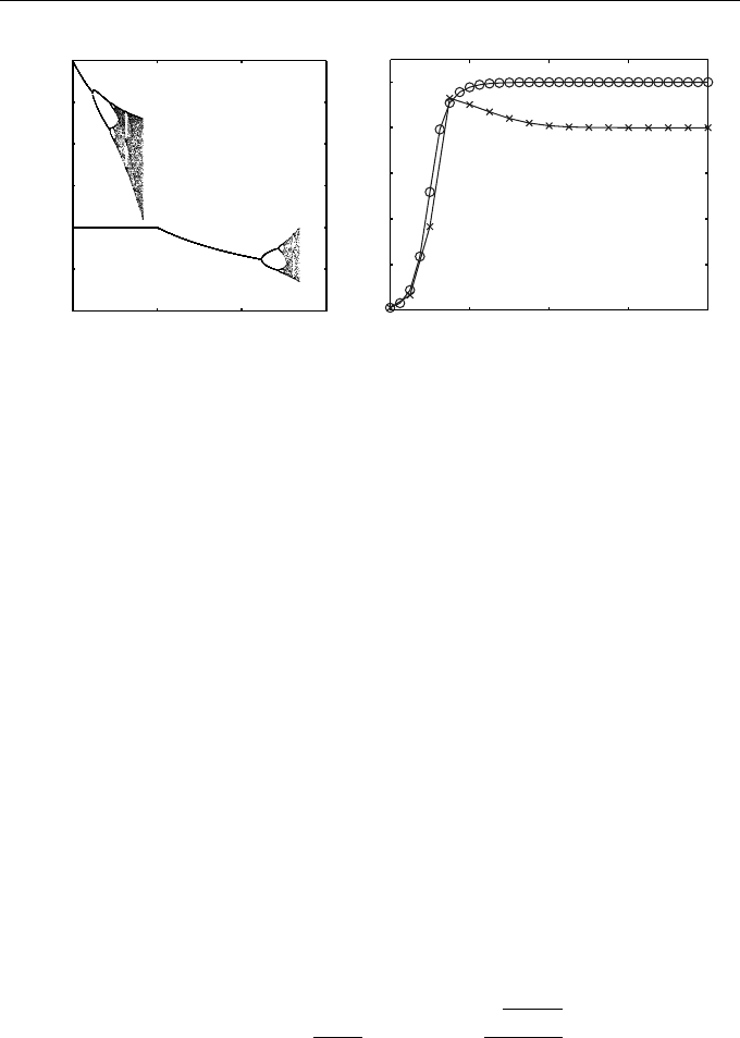
These results are conﬁrmed by the bifurcation diagram shown in Figure 12.2

(left). There is some cause for some concern, since the numerical method has

linearly stable ﬁxed points (x

∗

and x

∗

) that are not ﬁxed points of the ODE—

they are so-called spurious ﬁxed points—and so numerical experiments could

lead to false conclusions being drawn regarding the dynamical properties of the

system being simulated. However, since these spurious ﬁxed points depend on

h they may be detected by repeating the simulation with a diﬀerent value of

h—any appreciable change to the ﬁxed point would signal that it is spurious.

The results of such an e xperiment are shown in Figure 12.2 (right) where the

solution reaches the ﬁxed point x

∗

= 1/h = 0.8 when h = 1.25, but when h is

reduced to 0.625 it approaches the correct ﬁxed point x

∗

= 1.

When the ﬁxed points x

∗

and x

∗

lose stability as h is increased there ap-

pears to be a sequence of period-doubling bifurcations similar to those observed

in the previous example—the dynamics become to o complicated for us to sum-

marize here. The occurrence of spurious ﬁxed points is not restricted to the

modiﬁed Euler method—it is common to all explicit RK methods. A more de-

tailed investigation of the dynamical behaviour of RK methods is presented in

Griﬃths et al. [25].

When f (x) is a polynomial of degree d in x, then f(x +

hf(x)) will be a poly-

nomial of degree d

174 12. Long-Term Dynamics

0.5 1 1.5 2

0.5

1.5

2.5

, 500 < n < 520

0 5 10 15 20

0.2

0.4

0.6

0.8

h = 1. 25

h = 0. 625

Fig. 12.2 A bifurcation diagram for the modiﬁed Euler method applied to

the logistic equation of Example 12.4 is shown on the left. On the right are

individual solutions from the method with h = 1.25 (×) and h = 0.625 (◦)

EXERCISES

12.1.

Show that the system

(t) = y(t) − y

(t),

(t) = x(t) − x

(t)

(12.14)

has four ﬁxed points and investigate their linear stability. (A phase

portrait of solutions to this system is shown in Figure 13.4 (right).)

12.2.

Prove the ﬁrst part of Theorem 12.9. That is, prove that f (x

∗

) = 0

implies that F (x

∗

) = 0 and vice versa when f and F are related via

(12.8).

12.3.

If m × m matrices A and B are related via B = I + hA, prove

that they share the same eigenvectors and that the corresponding

eigenvalues are related via λ

= 1 + hλ

12.4.

Verify, by substitution, that the diﬀerence equation (12.10) has a

solution of the form x

= a + (−1)

b, where

a =

1 + h

and b =

√

− 1

which is real for h > 1.

12.5.

Verify the expressions (12.12) for the ﬁxed points and (12.13) for

the Jacobian in Example 12.11.

Exercises 175

12.6.

Repeat the calculations of ﬁxed points and their linear stability

in Example 12.11 for the function f(x) = αx(1 − x), where α is a

positive constant. Check your results with those given in the example

when α = 2.

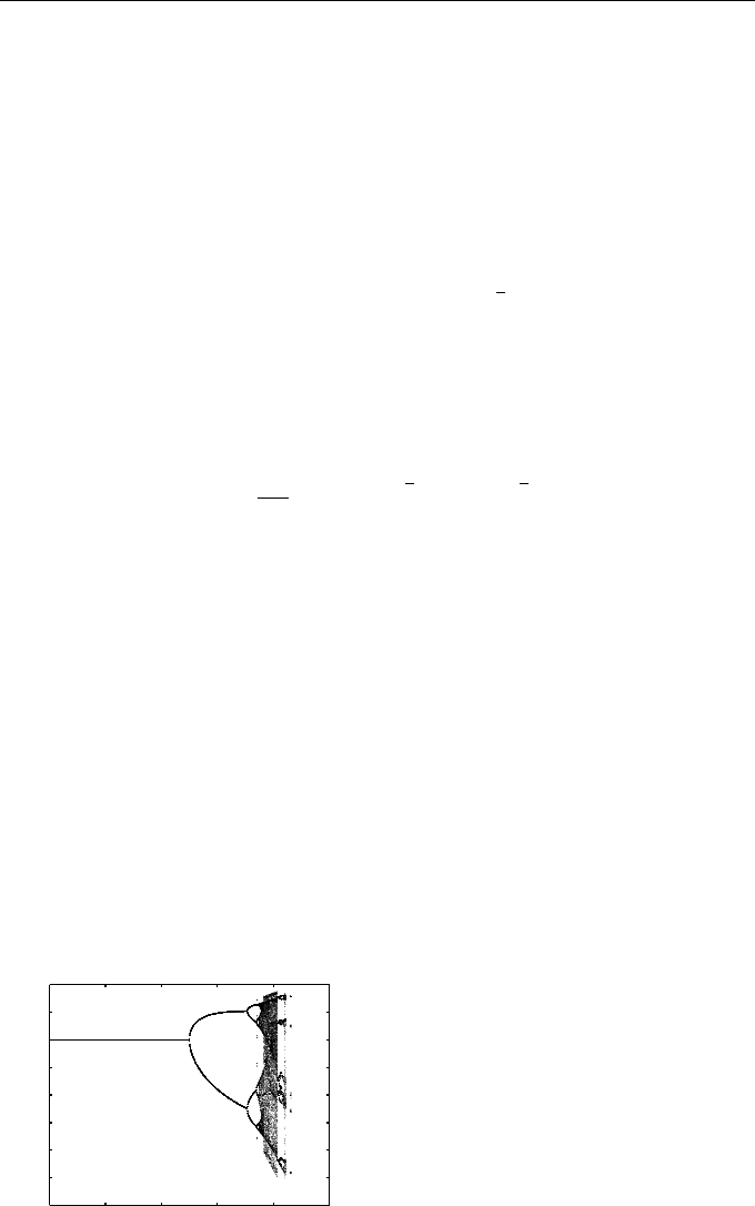
12.7.

???

Consider the AB (2) method (4.10) applied to the scalar equation

(t) = f (x(t)). Show that this may be written in the form of the map

(12.7) by deﬁning y

= x

n+1

, z

= x

(which implies z

n+1

= y

)





, and F (x

) =





3f(y

) − f(z

)





In the case f(x) = 2x(1 − x), show that there are two ﬁxed points

∗

= [0, 0]

and x

∗

= [1, 1]

Verify that the Jacobian of the map is given by

∂F

∂x

(x) =



1 +

(y) −

(z)

1 0



and, hence, investigate the linear stability of the ﬁxed points. Do

your results agree with the bifurcation diagram shown in Fig-

ure 12.3?

12.8.

Supp ose the separable Hamiltonian problem (see (15.14))

(t) = −V

(q),

(t) = T

(p)

is s uch that V

(0) = T

(0) = 0, V

(0) > 0 and T

(0) > 0. Show

that the Jacobian at the equilibrium point p = q = 0 has purely

imaginary eigenvalues.

0 0.2 0.4 0.6 0.8 1

−0.2

0.2

0.4

0.6

0.8

1.2

1.4

Fig. 12.3 Bifurcation diagram for the

AB(2) method applied to the logistic

equation of Exercise 12.7