Kallen A. Understanding Biostatistics

Подождите немного. Документ загружается.

120 LEARNING ABOUT PARAMETERS, AND SOME NOTES ON PLANNING

5.2 Test statistics described by parameters

The principal task of statistics is to reduce data to something that is interpretable. We see

our data, which are observations of an outcome variable, as a representative sample from a

hypothetical inﬁnite population in which the corresponding data are described by a distribu-

tion function. This distribution is speciﬁed up to a few unknown parameters. For example,

the ubiquitous Gaussian distribution depends on the parameter vector θ = (m, σ

), where m

is the mean and σ

the variance. For the purpose of this discussion we will denote a general

distribution function by F (x, θ), where θ may be a parameter vector, but will still be called

a parameter. The aim of the statistical analysis is to estimate this parameter using an esti-

mator, which itself has a distribution because its value varies with the sample we draw from

the population.

Since this will be a discussion about tests, our primary interest is not in the CDFs that

describe the population data, but in the CDFs of test statistics (which are summaries of the

sample data). In such a case the parameter θ may be multidimensional and contain one part

that is of interest (such as the odds ratio) but also some nuisance parameters. For example, if

we want to test for a mean difference (our parameter of interest) in Gaussian data, the original

model also contains a nuisance parameter, the variance. Such nuisance parameters cannot be

ignored; a way to handle them must be found (this is how the t distribution emerges: we use

a particular estimate for the variance, which replaces the original Gaussian distribution by a

t distribution). To simplify the present discussion we suppress any nuisance parameters from

the notation, so that the CDF F (x, θ) of the test statistic contains only one parameter. The

null hypothesis of the test we are interested is written θ = θ

, where θ

is a speciﬁed value

of the parameter, usually zero or one. This means that the distribution F(x) under the null

hypothesis is the same as F(x, θ

When it comes to the parameter θ, statistics addresses two different problems. The ﬁrst is

what we actually know about θ, and the second is what is the best estimate of θ. These two

problems must not be confused: a small sample may produce an accurate estimate, but our

conﬁdence in it may still be rather low. The two problems can be described as follows.

Hypothesis testing. We want a test of the hypothesis that θ = θ

. The conﬁdence in the

rejection of this hypothesis is inferred from the p-values which we compute from the

distribution F (x, θ

). For our discussion we mostly assume that this test is one-sided

and that the p-value is computed from the value x

∗

of the test statistic X obtained in

the experiment as the probability P(X ≥ x

∗

|θ

), that is,

p = 1 − F (x

∗

−,θ

The different p-values based on this observation, as a function of θ

, are what constitute

the conﬁdence function.

Parameter estimation. This is about ﬁnding the ‘best’ value for θ, based on the informa-

tion the data give us. One estimation method is the likelihood method, which addresses

the problem by asking, given the data we have, what is the most likely value of θ.

Mathematically this means that we want to ﬁnd the θ that maximizes the probability

L(θ) for what we have observed. We do not use L(θ) as a true probability, and it is

therefore referred to as the likelihood function of θ. The estimation method is called the

maximum likelihood method. Though probably the most important estimation method,

TEST STATISTICS DESCRIBED BY PARAMETERS 121

Box 5.1 On Bayes, Fisher and the maximum likelihood concept

The maximum likelihood theory was created single-handedly by R. A. Fisher between

1912 and 1922, culminating in his fundamental paper ‘On the mathematical foundations

of theoretical statistics’. Prior to this time most statistical reasoning had been based on

Bayes’ theorem which gives the posterior CDF P(θ|x) for θ from the CDF F (x, θ)of

the test statistics and a prior distribution Q(θ) for the parameter as

dP(θ|x) ∝ dF (x, θ)dQ(θ).

Here x is the observed data, and the proportionality constant makes the integral one. In

the nineteenth century the terminology was that dF(x, θ) was a direct probability (for

the outcome x,givenθ) and dP(θ|x) an ‘inverse probability’ (for θ, given the observation

x). Laplace, at least, used the terminology that θ was the cause and x the effect, and

looked for the most probable cause based on the observed effect. Most statistics was

done under the assumption that dP (θ|x) ∝ dF (x, θ), which means that a uniform prior

(dQ(θ) = dθ) was used. The major argument against such a choice of prior in the

physical sciences is that nature does not randomly select parameter values, but even if

you accept the argument about the prior (which Fisher did not) the integrals involved

in probability statements about θ are still complicated to compute in many cases, and

Fisher therefore maximized the direct probability instead. With this he eliminated all

reference to a subjective prior distribution, an idea Fisher hated. This led to a confusion

of terminology which was not cleared up until 1921 when Fisher introduced the term

‘likelihood’ for the density/probability function dF (x, θ) when considered as a function

of θ, given data. A year later he also introduced the term ‘maximum likelihood estimate’.

This constitutes the birth of the frequentist school of statistics.

On many occasions frequentists need to replace the log-likelihood with what is

called a penalized log-likelihood in order to get sensible parameter estimates. Such

a likelihood is obtained by subtracting from the log-likelihood a penalty function

φ(θ

). Put in the context above, this corresponds to having a prior density of the form

dQ(θ) = e

−φ(θ)

dθ.

it is not the only one. For a short discussion on how this concept is connected with the

Bayesian approach to statistics, see Box 5.1.

Knowledge about a parameter θ is derived from the distribution F(x, θ) of the test statistic

with the observed value of the test statistic inserted, and not directly from the likelihood

function. However, in many cases there is a close connection between these, because we use

the likelihood method to derive the test statistic, and then the approximation of the distribution

for this is derived from the likelihood function.

To pursue the question of what we know about the parameter, if we want to test if

θ = θ

at a particular signiﬁcance level α, we ﬁrst compute the (one-sided) p-value and then

compare it to our chosen α. Alternatively, we can ﬁrst determine the critical value x

crit

deﬁned

by the relation

1 − F (x

crit

−,θ

) = α,

122 LEARNING ABOUT PARAMETERS, AND SOME NOTES ON PLANNING

and then reject the hypothesis when the observed value x

∗

of the test statistic is such that

∗

≥ x

crit

. The set of outcomes {x ≥ x

crit

}deﬁnes a region in the space of test outcomes, which

is referred to as the critical region for the test. How to modify this for one-sided tests in the

other tail and for two-sided tests is left to the reader. The implicit assumption is that there is one

particular value, θ

true

, which is such that the true distribution of the test statistic is F(x, θ

true

(This distribution was denoted G(x) in Section 4.5.2.) Once we have obtained the data from

the experiment we can estimate θ

true

and also describe what we actually know about it.

5.3 How we describe our knowledge about a parameter from

an experiment

Suppose that we have performed an experiment and have obtained the value x

∗

for the test

statistic. The distribution of the test statistic is assumed to depend on a parameter θ such that

large values of θ correspond to large values of the test statistic. Traditionally the knowledge this

observation provides us with about θ is summarized in a conﬁdence interval with a speciﬁed

conﬁdence level 1 − α. As mentioned in Section 4.6.1, when we discussed a single binomial

parameter, such an interval has the interpretation that in the long run a fraction 1 − α of them

will contain the true parameter θ

true

. Not all, only the fraction 1 − α. They have an intimate

relationship with p-values, and, in fact, it is all better explained by introducing the conﬁdence

function, from which both pieces of information can be deduced.

We deﬁne the (one-sided) conﬁdence function for θ by inserting the observed value x

∗

the distribution function for the test statistic

C(θ) = 1 − F (x

∗

−,θ).

The proper interpretation of this is as the proportion of experiments that will produce an

observation that is at least x

∗

when θ is the true value, which means it is the (one-sided)

p-value for that hypothesis. This function summarizes the knowledge we obtain about the

true parameter value from the observation x

∗

One important special case is when we have a location model, which means that we have

that F (x, θ) = F(x − θ) for a CDF F (x) of one variable. If we introduce the notation θ

∗

= x

∗

we can in this case

write

C(θ) = 1 − F (θ

∗

− θ) = F (θ − θ

∗

so the conﬁdence function is obtained from the CDF under the null hypothesis (which is

F (x)) by a horizontal shift of magnitude θ

∗

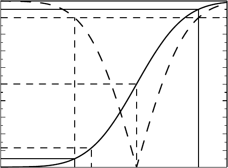
. Such a function may look like the solid curve in

Figure 5.1. This plot shows how we derive p-values and conﬁdence intervals from C(θ):

•

The value C(θ

) gives the p-value for the null hypothesis θ ≤ θ

(In Figure 5.1 this

takes the value 0.12.)

•

1 − C(θ

) deﬁnes the p-value for the hypothesis θ ≥ θ

As long as the distribution is continuous, otherwise we replace θ

∗

in the middle by its left-hand limit.

We use the notation θ ≤ θ

to denote the situation where the null hypothesis is θ = θ

and the alternative is

θ>θ

, with a similar convention for the opposite one-sided hypothesis.

OUR KNOWLEDGE ABOUT A PARAMETER FROM AN EXPERIMENT 123

0.1

0.2

0.3

0.4

0.5

0.6

0.7

0.8

0.9

Conﬁdence function C (θ)

Population parameter θ

Figure 5.1 The conﬁdence function based on the observed statistical result θ

∗

. The solid

curve shows the one-sided conﬁdence function, whereas the dashed curve corresponds to the

two-sided one. See text for details.

•

Taking the inverse image of an interval of length d on the y-axis, we obtain a conﬁdence

interval for the parameter θ with conﬁdence level d. In the graph there is a symmet-

ric 90% conﬁdence interval (θ

,θ

) around θ

∗

, obtained by ﬁnding the points on the

θ-axis with conﬁdence function values equal to 0.05 and 0.95 (i.e., C(θ

) = 0.05 and

C(θ

) = 0.95, respectively).

We noted in Section 4.5.2 that for symmetric two-sided conﬁdence statements (which

conﬁdence intervals typically are) we can use the distribution function of the square of

the test statistic. Since many one-sided tests are based on the Gaussian distribution, this

means using the χ

distribution (see Appendix 5.A.2). We will use the notation χ

(x) for

the CDF of the χ

(n) distribution. This is illustrated in Figure 5.1, where the dashed curve

shows the conﬁdence function for two-sided alternatives. Inspecting it, we ﬁnd that (1) the

estimate θ

∗

corresponds to the minimum, and (2) the 90% conﬁdence interval for θ is

obtained by reading off where the dashed curve intersects the line y = 0.9 (the horizon-

tal dashed line). The one-sided conﬁdence function is the one with most information,

because when we square, we lose track of the sign, but the two-sided version is required in

many problems.

A ﬁrst illustration of this was given in Section 4.6.1, to which we want to add two further

examples, both of which are concerned with one-parameter problems. In the next section we

will address the more complicated problem with two parameters when we are only interested

in some particular combination of these, which will leave us with one nuisance parameter.

Example 5.1 This is a continuation of the Fisher’s exact test discussed in Section 4.5.1

and uses the data of the ﬁrst study there. Fisher’s test can be expressed as a test of the

null hypothesis that the odds ratio is one, and we now want to exploit this test further in

124 LEARNING ABOUT PARAMETERS, AND SOME NOTES ON PLANNING

0.1

0.2

0.3

0.4

0.5

0.6

0.7

0.8

0.9

Conﬁdence Function

54321

Odds Ratio

0.04

0.08

0.12

P(x

= 67)

5432

Odds Ratio

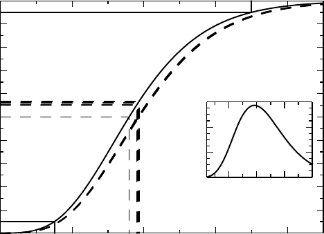
Figure 5.2 The exact conﬁdence function for the odds ratio for the ﬁrst Hodgkin’s lymphoma

table is shown as the solid curve, whereas some approximations based on natural estimates of

the odds ratio are shown as the almost overlapping dashed curves – see text. The inset graph

shows the likelihood function that determines the maximum likelihood estimate.

order to obtain knowledge about the true odds ratio from available data. What we do is

essentially to repeat Fisher’s test for arbitrary values θ of the odds ratio. For each θ we compute

the probability that the observation is 67 or larger, which gives us the conﬁdence function

C(θ) that is plotted as the solid curve in Figure 5.2. Also illustrated is the symmetric 95%

conﬁdence interval for the odds ratio, which is (1.75, 4.49), and is indicated by the solid lines in

Figure 5.2.

There is more to be said about this example, also illustrated in Figure 5.2. The computation

of the conﬁdence interval for the odds ratio was done without reference to a point estimate.

How we obtain a point estimate of the odds ratio is a separate question. There are quite a few

options available.

•

One estimate would be the point that gives 50% conﬁdence, that is, the solution of the

equation C(θ) = 0.5. In our case this point estimate is 2.79.

•

Intuitively the most obvious choice is probably the empirical odds ratio which was

discussed at the end of Section 4.5.1, which we know is 2.93.

•

A further choice is to use the θ for which the observed count equals the expected count.

This is the θ which solves the equation x

∗

= E

) and gives us the estimate 2.92.

•

A ﬁnal choice is to use the maximum likelihood estimate, which in this case is 2.90.

All these estimates are shown in Figure 5.2, where we see that all but the ﬁrst of these estimates

correspond to more than 50% conﬁdence on the solid curve. We also see that the variability

for the other three estimates is very small. Each of these suggested point estimates for the

OUR KNOWLEDGE ABOUT A PARAMETER FROM AN EXPERIMENT 125

odds ratio has its own rationale and to each of them there is associated a conﬁdence function,

also indicated in Figure 5.2 as the dashed curves. These conﬁdence curves agree well with

each other, but not with the original, solid, one. Why this is will be explained after we have

discussed how the alternative conﬁdence functions are obtained.

As can be seen from the discussion in Appendix 5.A.1, and will be further detailed in

Example 13.3, under the assumption of a (non-central) hypergeometric distribution for x

we have that if

θ is the empirical odds ratio, then

ln(

θ) ∈ AsN



ln(θ),

− μ

− r + μ



where μ = E

) and r is the column sum we condition on. Inserting the observation x

∗

for μ provides us with an approximative conﬁdence function for the odds ratio, based on the

empirical odds ratio. With our data we have that the estimated log-odds ratio is 1.076, and its

variance is estimated as 1/67 + 1/34 + 1/43 + 1/64 = 0.083. This gives a 90% conﬁdence

interval of (0.602, 1.551) for the logarithm of the odds ratio, which upon exponentiation gives

the corresponding interval for the odds ratio as (1.82, 4.71).

The next choice for an estimate of the odds ratio in the list above is the solution θ of

the equation x

∗

= E

). For this estimator we can obtain an approximative conﬁdence

function (by appealing to large-sample theory) as

C(θ) = 



) − x

∗

√

)



How to compute the mean and variance is discussed in Appendix 5.A.1.

Finally, we have the maximum likelihood approach, in which we compute, for different

values of the odds ratio θ, the probability of obtaining exactly the observed value 67. This

gives us a function of θ which is illustrated in the inset graph in Figure 5.2, a function which

has its maximum at the point 2.90, which therefore is the maximum likelihood estimate. (The

general method of obtaining the conﬁdence function for a maximum likelihood estimator is

the subject of Section 13.3.)

It remains to explain why the dashed curves differ from the solid one in Figure 5.2. This

explanation has less to do with the fact that the three alternatives build on approximations,

appealing as they do to large-sample theory. The root cause of the difference is the discrete

nature of the hypergeometric distribution. In this case we have not used the mid-P adjustment

in equation (4.2), which we did for the binomial parameter in the previous chapter. With

the mid-P adjustment the solid curve moves to the dashed ones, and the conﬁdence interval

with it.

The next example describes another one-parameter problem.

Example 5.2 We wish to study a certain adverse event, which is likely to occur with long-

term treatment using a particular drug. In order to estimate the risk for this adverse event,

we planned to follow 20 subjects for 5 years. The actual observation times for the patients

varied between 4.4 and 6.9 years and the event occurred during this observation period in

12 out of the 20 subjects. This particular adverse event can appear anywhere during treat-

ment, so we assume there is a constant hazard λ for it. If subject i is observed for time

, the probability that he experiences the event while being observed is p

(λ) = 1 − e

−λT

Denote by x

the outcome for subject i: it is one if the event has occurred, otherwise zero.

126 LEARNING ABOUT PARAMETERS, AND SOME NOTES ON PLANNING

0.2

0.4

0.6

0.8

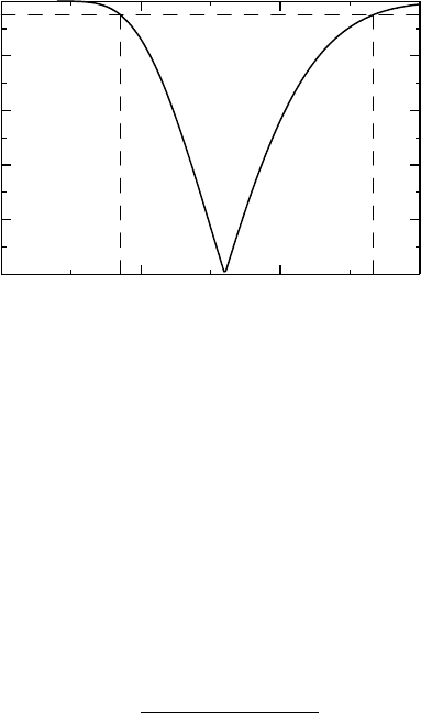
Conﬁdence function C (λ)

0.10 0.2 0.3

Hazard rate λ

Figure 5.3 Two-sided conﬁdence function for a hazard rate.

The total number of events, x = x

+ ...+ x

, is not an observation of a binomial distribu-

tion, even though each x

is an observation of a Bin(1,p

(λ)) distribution. We can, however,

still appeal to the CLT to ﬁnd that the total number of events is asymptotically Gaussian in

distribution:

x =



i=1

∈ AsN





(λ),



(λ)(1 − p

(λ))



From this we derive the two-sided (approximate) conﬁdence function

C(λ) = χ



(x −



(λ))



(λ)(1 − p

(λ))



We estimate λ as the value λ

∗

for which C(λ) = 0 (i.e., solve



(λ) = x) and obtain

conﬁdence limits for λ as shown in Figure 5.3. We see that the hazard is estimated as 0.16

with 95% conﬁdence interval (0.09, 0.27). We can also compute the predicted probability

that an individual experiences an adverse event within 5 years as 1 − e

−5·0.16

= 0.55, with

corresponding 95% conﬁdence interval (0.35, 0.74).

We have used the conﬁdence function in a way that makes it only a graphical tool for

obtaining conﬁdence intervals and p-values. We have tacitly assumed that we are only dealing

with situations in which such things can be computed. However, looking at the one-sided

conﬁdence curve in Figure 5.1 it is tempting to see it as a CDF for the parameter θ and,

subsequently, make probabilistic statements about θ. There are two problems with this:

1. There is in general no guarantee that the one-sided conﬁdence function is monotonically

covering the entire interval (0, 1), which is a necessary condition for it to be a CDF.

2. There is a considerable conceptual leap involved in assigning a probability to θ. What

the conﬁdence function does is to assign probabilities to where we ﬁnd θ, which is

fundamentally different.

STATISTICAL ANALYSIS OF TWO PROPORTIONS 127

We will encounter a famous example of the ﬁrst problem later, in Example 7.7. When it

comes to the second problem, we may note that Fisher himself argued for such a probabilistic

viewpoint. He did this in 1930, three years before Kolmogorov formulated his axioms for

probabilities and four years before Neyman introduced the concept of the conﬁdence interval.

Fisher also assigned a special name to this probability, ﬁducial. He set about introducing it

by ﬁnding a substitute for the subjective priors used in Bayesian theory. Fisher had a distaste

for subjectivity and wanted probabilistic statements derived from objective data only. The

concept led to a lot of controversy and more or less died with Fisher himself. As already

indicated, there are situations where very speciﬁc assumptions on the prior in the Bayesian

approach are equivalent to this ﬁducial probability, the prime example being the t-test (and

shift models in general).

The controversy around ﬁducial probabilities is better left to the theoretical statisticians;

we only use the conﬁdence function as a convenient tool to summarize the knowledge obtained

from an experiment. It is, however, interesting to note that the difference between using the

conﬁdence function and using conﬁdence intervals is essentially a continuation of the debate

about the nature of the p-value outlined in Box 1.3; the conﬁdence function is much closer

to the view advocated by Fisher, whereas a single conﬁdence interval, with its prespeciﬁed

conﬁdence level, is more of a Neyman–Pearson tool for decision making.

5.4 Statistical analysis of two proportions

5.4.1 Some ways to compare two proportions

For a more complicated situation where we want to derive conﬁdence about a parameter,

we next discuss ways to compare two proportions. We assume we have observations x

i = 1, 2, of two independent binomial distributions Bin(n

), respectively, and we want to

compare p

and p

. For the purposes of the discussion we assume that the ﬁrst group consists

of individuals exposed to something, and the second group is a control group. We want to

summarize the group comparison in a single parameter, which we denote θ in general. The

most important choices for θ are:

1. the difference  = p

− p

, which measures the additive contribution of the exposure;

2. the relative ratio RR = p

, closely related to the relative contribution of the expo-

sure (p

− p

)/p

= RR − 1;

3. the odds ratio OR = p

(1 − p

)/[p

(1 − p

)], which is the ratio of the odds for the

two groups.

(We may note in passing that the odds ratio can be written as a relative risk, because (by

independence)

OR =

P(X

= 1 and X

= 0)

P(X

= 0 and X

= 1)

P(X

)

P(X

)

It is therefore the relative probability of obtaining a larger value on the ﬁrst variable, to that of

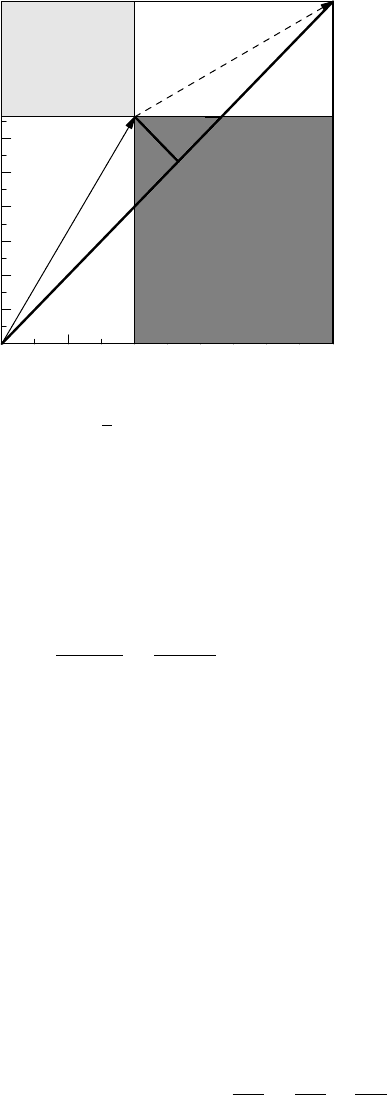
a smaller. This is a formulation that can be extended to more general data.) The three measures

discussed above are geometrically described in Figure 5.4, and are the ones we will focus on.

There are, however, other useful combinations of p

and p

128 LEARNING ABOUT PARAMETERS, AND SOME NOTES ON PLANNING

0.1

0.2

0.3

0.4

0.5

0.6

0.7

0.8

0.9

0.20 0.4 0.6 0.8 1

, p

)

|Δ |/

√

Figure 5.4 Geometrical illustration of parameters comparing two binomial probabilities.

RR is the slope of the solid arrow, ||/

√

2 the distance to the identity line, and OR the ratio

of the dark gray to the light gray rectangle (we can also see it as the ratio of the slopes RR

and RR

= (1 − p

)/(1 − p

)).

Example 5.3 If we measure the frequency of a particular outcome in an exposed and an

unexposed group, respectively, we get the attributable fraction among those exposed as

− p

RR − 1

This measures the proportion of cases that would be eliminated if we eliminated the exposure,

should those in the exposed group have the same risk for being a case as those in the unexposed

group (see Box 5.2). Related to the attributable fraction is the excess risk q, which is the

probability that an exposed individual becomes a case, had he not been one when unexposed,

which means that it is derived from the equation p

= p

+ q(1 − p

)orq = (p

− p

(1 − p

Another alternative transformation of p

and p

is the number needed to harm, which

refers to how many individuals we need to expose in order to get one extra case. It is deﬁned by

the relation N · = 1 and is therefore given by the inverse of . It is often used by clinicians

as a way to quantify risks. However, it is a measure with drawbacks. Suppose we have two

different exposures with probabilities p

and p

and let p

denote the risk for an unexposed

individual. Then the extra risk of the ﬁrst exposure over the second exposure is the difference

of the risk differences to the unexposed, but the relation for the numbers needed to harm is

more complicated:

− p

= (p

− p

) − (p

− p

) ⇔

−

STATISTICAL ANALYSIS OF TWO PROPORTIONS 129

Box 5.2 The attributable risk in the population

The attributable risk, also known as the etiologic factor (or fraction) is a widely

used measure for assessing the public health consequences of an association between

an exposure (E) and a disease (C). It was ﬁrst introduced by Morton B. Levin in

1953 as a way to quantify the impact of smoking on lung cancer occurrence, and is

deﬁned as

AR =

P(C) − P(C|E

)

P(C)

It measures the proportion of disease cases that can be related to the exposure, and

can therefore be used to assess the potential impact of a prevention program. It takes

into account both the strength of the association between exposure and disease, and the

prevalence of the exposure. It should be recognized that it assumes that the probability

of the disease in an exposed subject when the exposure is removed is the same as that

for an unexposed subject, an assumption we can seldom prove.

If we replace P (C) with P(C|E) we get the attributable risk AR(E) among those

exposed. Its relation to the attributable risk is that the latter is obtained by multiplying

by the proportion of those with the disease that has been exposed:

AR = AR(E)P(E|C).

This is derived using Bayes’ theorem. For rare diseases we can estimate AR from a

case–control study, if we approximate the relative risk with the odds ratio.

where N

denotes the numbers needed to harm comparing groups a and b. This property

makes it doubtful that this parameter really is easily interpretable. When the event is positive

we talk about the number needed to treat (NNT).

In order to build the statistical machinery for the analysis of any of the parameters discussed

above, we start from the large-sample N(p, p(1 − p)/n) approximation for the distribution

of the estimator ˆp = x/n of p. This information can be used in two different ways. First, we

may note that

n(ˆp − p)

p(1 − p)

(x − np)

np(1 − p)

∈ χ

(1),

and since our two groups are independent, the sum of these expressions for the two groups

will have a χ

(2) distribution:

− n

)

(1 − p

)

− n

)

(1 − p

)

∈ χ

(2).

How to use this observation in order to derive conﬁdence statements about different functions

of p

and p

will be discussed in Section 7.7. That discussion will allow us to simultaneously

obtain conﬁdence information for any number of derived parameters we want. It is, however,

more involved mathematically than the approach we will discuss here.