Kallen A. Understanding Biostatistics

Подождите немного. Документ загружается.

100 THE ANATOMY OF A STATISTICAL TEST

Box 4.6 Distributions symmetric around zero

One of the key properties of the standard normal distribution is that it is symmetric

around x = 0, which means that its probability density has the same value at the two

points ±x for all x. Expressed in terms of the CDF this means that

F (−x) = 1 − F(x−), (4.1)

which is equivalent to the probabilistic statement that it is as probable to get an obser-

vation to the left of −x as it is to get one to the right of x: P(X ≤−x) = P (X ≥ x).

0.1

0.2

0.3

0.4

0.5

0.6

0.7

0.8

0.9

−3 −2 −1 3210

y = 1 − F(x)

y = F(x)

y = f(x)

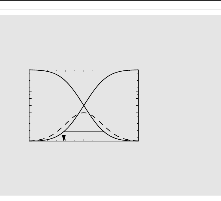
The ﬁgure above explains why equation (4.1) expresses symmetry around zero

for a continuous distribution (in fact, for a Gaussian distribution). The dashed func-

tion is the density function and we see that F (x) is the same as the reﬂection in the

y-axis of 1 − F (x). The rectangle at the bottom illustrates that the symmetry relation in

equation (4.1) at the point x = 1.1.

using the square X

as the test statistic instead, because the two-sided test for X becomes a

one-sided test for X

. For the normal distribution this turns the problem into one involving a

chi-square distribution (see Appendix 5.A.2).

Just as there may be more than one way to detect a speciﬁc chemical in a ﬂuid, so the

same data can often be approached by different statistical tests. First of all, we can deﬁne

different test statistics. If we choose to do a t-test, our test statistic is based on a mean

difference, whereas the corresponding non-parametric test, the Wilcoxon test, is based on

a rank sum. But also when we have decided on the test statistic there are sometimes a few

options in the details of the computation of the p-value. A further aspect of statistical testing

is concerned with choosing between an unconditional and a conditional tests. An example is

Fisher’s exact test for a 2 × 2 table, discussed above. It starts with two binomial distributions

(the two rows) and we consider the result conditional on the outcome of the ﬁrst column total.

This way we reduce two parameters, the two binomial proportions, to one, the odds ratio.

The general situation is that we are interested in a parameter (say, the odds ratio) and there

are other so-called nuisance parameters in the distributions (the ﬁrst binomial proportion,

for example). It is then sometimes possible to derive a conditional distribution which deﬁnes

a distribution (under the null hypothesis) without the nuisance parameters. The down-side

MAKING STATEMENTS ABOUT A BINOMIAL PARAMETER 101

of this is that such a test is a conditional test, conditional on the value of this other test

statistic. Even though the other test statistic has nothing to do with our primary problem, it

is still the case that any p-value will be computed under the assumption that this other test

statistic takes on a particular value. Statisticians are divided as to how much this allows us

to generalize (most medics probably do not care). For Fisher’s exact test, can you generalize

to all 2 × 2 tables that can be derived from this experiment, or only to those that have the

same margins?

4.6 Making statements about a binomial parameter

4.6.1 The frequentist approach

We now wish to address what appears at ﬁrst to be a very simple problem. Suppose that we

have studied n = 101 individuals and found that x = 67 of these have a particular property;

what we can say about the binomial parameter p which is the fraction of individuals in

the population with this property? That we have the point estimate p

∗

= 67/101 = 0.66

of p is obvious, but what can we say about how accurate this estimate is? A discussion

about this simple problem will allow us to compare the frequentist and Bayesian approaches

to statistics.

Here is how the frequentist approaches the problem. He bases his analysis exclusively on

what he knows. If p is the true parameter value, the number of individuals in the sample with

the property has the Bin(n, p) distribution. The CDF for this distribution is given by

F (x, p) =



k≤x





(1 − p)

n−k

which, like the hypergeometric distribution in the previous section, is a step function. We can

then deﬁne the function (where x is the observed outcome)

C(p) = 1 − F(x−,p),

which is the probability P(X ≥ x|p) that we get an observation at least as large as the observed

value x, when the true parameter value is p. This function C(p) is an increasing function, start-

ing at zero when p = 0 and ending at one when p = 1. It is called the conﬁdence function for

the binomial parameter p based on the outcome of this experiment. From the frequentist’s point

of view this function contains all the information about p that is provided by the experiment.

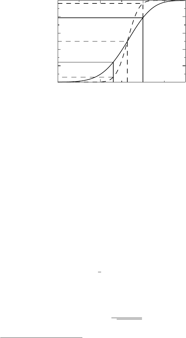
For the data above, the conﬁdence function C(p) is illustrated as the solid curve in Figure 4.3.

The graph also contains a dashed curve, which shows what the conﬁdence function would

look like if we had ﬁve times as many observations but with the same observed proportion

(i.e., 335/505). We have added this curve to illustrate how a larger sample size increases the

knowledge about p, by making the conﬁdence curve steeper.

What can the conﬁdence function tell us about the binomial parameter p? First, we note

that the point estimate 0.66 corresponds to the conﬁdence value 0.5 for both conﬁdence

curves (because we assumed that we had the same point estimate in the two cases). Next we

consider the solid conﬁdence function. For this we have that C(0 .63) = 0.24, which means

102 THE ANATOMY OF A STATISTICAL TEST

0.2

0.4

0.6

0.8

Conﬁdence in p

0.5 0.6 0.7 0.8

Binomial parameter p

Figure 4.3 Two conﬁdence functions for a binomial parameter, where the dashed one has

ﬁve times as many observations as the solid one.

that this is the one-sided p-value if we test the hypothesis that p ≤ 0.63.

Similarly, we have

C(0.70) = 0.79, so the one-sided p-value for the test of the hypothesis p = 0.70, or larger, is

0.21. In this way we can compute the p-values, for all kinds of one-sided hypotheses regarding

the parameter p.

The numerical observations above also mean that the interval (0.63, 0.70) is a conﬁdence

interval with conﬁdence level 0.55 (= 1 − (0.24 + 0.21)). A conﬁdence interval has con-

ﬁdence degree 1 − α, if the method we use to compute it guarantees that it contains the true

value p in the fraction 1 − α of experiments. We will discuss such intervals in more detail in the

next chapter. The corresponding p-values for conﬁdence functions based on the larger sample

size can be read off from the dashed curve as C(0 .63) = 0.060 and 1 − C(0.70) = 0.036, so

in this case the same interval has conﬁdence level 0.904.

Actually, we have cheated a little here. There is a minor complication due to the discrete

nature of the binomial CDF F (x, p) as a function of x for ﬁxed p. The complication is that

P(X ≤ x) = F (x, p) but that P(X ≥ x) = 1

− F (x − 1,p),

which represents an asymmetry between the two tails, and justiﬁes why we should redeﬁne

C(p) as the compromise

C(p) = 1 −

(F (x − 1,p) + F (x, p)). (4.2)

This modiﬁcation is called the mid-P adjustment, and is actually the conﬁdence function

we have used above. It agrees to a very high precision with what we obtain if we apply a

large-sample approximation, namely

C(p) = 



np − x

√

np(1 − p)



. (4.3)

More precisely, the null hypothesis is p = 0.63 and the alternate hypothesis is p>0.63.

MAKING STATEMENTS ABOUT A BINOMIAL PARAMETER 103

Box 4.7 Conﬁdence intervals for a binomial parameter

The conﬁdence intervals we derive from the discussion in Section 4.6.1 are not the

ones most often used. The method discussed, for a symmetric conﬁdence interval of

conﬁdence degree 1 − α, is equivalent to ﬁnding the two solutions to the equation

∗

− p)

p(1 − p)/n

= z

α/2

, (4.4)

where z

denotes the (1 − α)th percentile for the standard Gaussian distribution. The

solution to this is given by

∗

α/2

1 +

α/2

√

n +

α/2

√



∗

(1 − p

∗

) +

α/2

These intervals were introduced in the late 1920s by Wilson, and differ from the standard

conﬁdence intervals, which are obtained by using the estimate p

∗

(1 − p

∗

)/n for the

variance and solving equation (4.4):

∗

± z

α/2



∗

(1 − p

∗

)

An important difference between the Wilson intervals and the conventional ones is that

the former are always restricted to [0 , 1]. In fact, it can be seen from the quadratic

equation that its limits are such that the interval for the odds p/(1 − p) is symmetrical

around the estimate on a multiplicative scale.

These are, however, only two of a number of different suggestions for how to

compute conﬁdence intervals for a binomial proportion. The exact version, called the

Clopper–Pearson intervals, is derived directly from the binomial distribution (without

the mid-P adjustment). It is conservative in terms of actual coverage level, a fact derived

from its discreteness. That reason, and the complexity of computing the exact interval

(prior to the computer age), has led to the emergence of a number of approximative

intervals, of which the standard one and the Wilson interval are only two.

This approximation is called de Moivre’s theorem and is justiﬁed in Section 4.7. (It is common

to use a mid-x adjustment instead of a mid-P adjustment to correct for the discreteness of the

binomial distribution, which means that the Gaussian approximation is computed not at the

point x but at the point x + 1/2. This is called a continuity correction or half-correction. We

will later see other arguments for why the mid-P adjustment might be the right thing to do.)

We have used a geometric approach to the description of how to derive knowledge about a

binomial proportion, but the algebra involved is discussed in Box 4.7 (using the large-sample

approximation).

At this point it is worth commenting on how to produce conﬁdence intervals for a

function of a parameter. Suppose we want to make statements about the odds p/(1 − p)

instead of about p itself. This is simple: all we need to do is to compute the conﬁdence

function as before and plot it, not versus p, but versus θ = p/(1 − p). Conﬁdence intervals

104 THE ANATOMY OF A STATISTICAL TEST

for the odds are derived in the same way as described above, which is equivalent to

applying the odds function f (p) = p/(1 − p) to the limits of the conﬁdence intervals

in Figure 4.3.

There are some interesting observations to make about this. To estimate θ from the ob-

servation x, the natural estimate is probably θ

∗

= x/(n − x), the empirical odds. But the

corresponding test statistic is not unbiased; its expected value is not θ. In fact, its mean value

does not even exist, because there is a positive probability of x/(n − x) becoming inﬁnite,

which occurs when x = n. However, for large n this is unlikely, unless p is very close to one,

and there is a useful approximation to the conﬁdence function, namely

C(θ) = 



ln(θ) − ln(θ

∗

)

√

1/x + 1/(n − x)



. (4.5)

In order to justify this, recall from basic calculus that ln(1 + x) ≈ x for small x, from which

we deduce that



n − x



≈ ln θ +

x − np

np(1 − p)

De Moivre’s theorem then implies that the right-hand side has (asymptotically) a Gaussian

distribution with mean zero and a variance given by

np(1 − p)

n(1 − p)

Finally, we replace np with the observation x and n(1 − p) with the observation n − x.

4.6.2 The Bayesian approach

We saw in Section 1.10 that the concept of probability is not restricted to probabilities

which can be interpreted as frequencies, and that there is a whole school of statisticians

who think of probabilities more in terms of an subjective assessment – the Bayesians. So

how would a Bayesian statistician approach the problem of obtaining knowledge about a

binomial parameter?

Before we discuss this, let us stress one particular aspect of the foregoing frequentist

analysis. The data from the experiment deﬁne a conﬁdence function, from which p-values and

conﬁdence intervals are derived. This type of conﬁdence is something that is very reminiscent

of a probability; it is always between 0 and 1, for a start. But its interpretation as a probability

is more involved. For example, for something to be a 90% conﬁdence interval means that if

we repeat the experiment very many times, we expect the true parameter to be somewhere

within these intervals in 90% of runs. It is not a probability statement about the parameter

but about the computational method for the interval. However, to make probability statements

about the parameter is precisely what Bayesian statisticians do. They do this following a

well-deﬁned process that captures the inductive aspect of science: we learn more as we do

more experiments.

Another point before we start the discussion is the need for a convenient notation that

conveys the important mathematical aspects of the discussion, which is about sums. To avoid

the conventional distinction between discrete and continuous stochastic variables we will use

the integral notation outlined in Box 4.8, which was also mentioned in Section 2.5. Now to

the Bayesian analysis.

MAKING STATEMENTS ABOUT A BINOMIAL PARAMETER 105

Box 4.8 Notation: Differentials and the Stieltjes integral

Statistics is often divided into a discrete and continuous version, with the former ex-

pressed in probability functions and sums and the latter having probability densities

and integrals (and therefore being more involved mathematically). In order to avoid this

distinction we will use a uniform notation based on the mathematical concept of the

Stieltjes integral.

If F (x) is a right-continuous function (in our case almost always a CDF), we denote

by dF (x) either the jump F(x) = F (x) − F (x−) at that point, if there is one, or the

differential at that point (we assume that a function that does not have a jump at a

point is differentiable there). The latter means that dF (x) = f (x)dx, where f (x)isthe

probability density at that point. At a jump point, the probability function is F (x). On

occasion we even let dF (x) denote the density f (x) at continuity points x.

Sums and conventional integrals are now replaced by the Stieltjes integral



g(x)dF (x).

This represents a sum – the notation



for an integral is actually only a slanted S for the

ﬁrst letter in sum – and the notation means that we sum the g(x) using weights dF (x).

It is deﬁned, by ﬁrst deﬁning it for a step function g(x) corresponding to the partition

a = x

<...<x

= b with values g

in the intervals (x

i−1

], as



g(x)dF (x) =



i=1

(F (x

) − F (x

i−1

)).

Repeating the standard deﬁnition of the Riemann integral (sandwich a general function

between two step functions with the same partition), we obtain, by making the parti-

tion ﬁner and ﬁner, a limit that deﬁnes the integral. For a continuous distribution with

dF (x) = f (x)dx, this is the conventional integral



g(x)f (x)dx, and if the distribution

is discrete, it is the sum



g(x

)F (x

Before he starts the experiment, the Bayesian statistician must have a prior opinion

about the value of the parameter p. In order to describe his prior belief he deﬁnes a CDF

Q(p), called the a priori distribution. If he is certain of the value of the parameter, he

should assign all probability to one point. The opposite extreme is complete ignorance, in

which case he might assign equal probability to everything between 0 and 1. We should

not confuse Q(p) with the heterogeneity distribution which was discussed in Section 2.5;

they are not related. The heterogeneity means that there are different probabilities for

different individuals, whereas the Bayesian assumes a common p for all, but is uncertain

about its value and wants that uncertainty to be propagated through the calculations.

Given the prior, the probability for obtaining a particular outcome is computed by

the formula

P(X = x) =



P(X = x|p)dQ(p),

106 THE ANATOMY OF A STATISTICAL TEST

where P(X = x|p) is the binomial probability function. The probability P(X = x) is called

the predictive probability for the different outcomes of the experiment.

Having decided on his prior opinion, the Bayesian statistician performs the experiment.

We assume he gets the same data as in the previous section (n = 101,x= 67 for a binomial

distribution). Using this information, he updates his belief about what p is. The updated

distribution F (p|x) is called the a posteriori distribution of p (based on the observation x)

and is obtained from Bayes’ theorem as

dF (p|x) =

P(X = x|p)dQ(p)

P(X = x)

= C(x)p

(1 − p)

n−x

dQ(p).

Here C(x) = 1/P (X = x) is independent of p and makes F (p|x) a CDF for p.

In case of complete certainty, when Q(p) has probability one at a single point, the a

posteriori distribution will also have probability one at that point; there is nothing in the

outcome of the experiment that will change your view.

There is a particular prior of special interest, called the uninformed prior (ﬂat or uniform

prior would probably be a better description). This is the prior distribution for which every

value of p in (0 , 1) is equally probable, and therefore means that dQ(p) = dp . Not surprisingly,

the uninformed prior implies that the predictive probability for all possible values is the same:

P(X = x) =







(1 − p)

n−x

dp =

n + 1

,x= 0,...,n.

Furthermore, the assumption implies that the a posteriori distribution becomes

dF (p|x) = (n + 1)p

(1 − p)

n−x

dp.

Such a distribution, for which the probability density f (p) is proportional to p

a−1

(1 − p)

b−1

is called the beta distribution with parameters a and b; we denote its CDF by β(p; a, b). We

therefore have that

F (p|x) = β(p; x + 1,n− x + 1).

The expected value for p based on this a posteriori distribution can be calculated as



pdF(p|x) =

x + 1

n + 2

, (4.6)

a result known as ‘Laplace’s rule of succession’ (see Box 4.9). As an application of this, if you

have no prior idea of what percentage of swans are white, you may assign the uninformative

prior to this. After having observed n swans, all white, your prediction is that the fraction

n/(n + 1) of all swans are white. (The frequentist would obtain this estimate had he seen n

white and one colored swans.) This is your inductive conclusion, and essentially means that

since you have only seen white swans, you believe most (or almost all, depending on n) swans

are white.

However, the point about Bayesian statistics is not really to use the uninformed prior.

The point is to synthesize prior knowledge into a more structured, but still subjective, prior

distribution Q(p). Assume that we believe that the true probability is somewhere in the vicinity

of 0 .4. To make it precise we assume that our subjective prior information can be summarized

MAKING STATEMENTS ABOUT A BINOMIAL PARAMETER 107

Box 4.9 Laplace rule of succession and the sunrise problem

If we have n independent observations of a Bernoulli experiment in which the event

has occurred k times, what is the probability that it will occur in the next, independent,

experiment? Conventional reasoning would estimate the unknown probability as k/n,

which therefore is the predicted probability that it will occur in the next test.

However, if we have had success on all occasions, so that k = n, is it obvious that this

is the proper estimate? The prediction would be that we are certain the event will occur

next time. But if we toss a possibly biased coin 10 times getting a head each time, is the

best predictive probability estimate really that we are certain to get a head next time?

Laplace addressed this as the sunrise problem: ‘what is the probability that the sun

will rise tomorrow?’ He argued as follows. Prior to knowing of any sunrises, one is

completely ignorant of the probability p of a sunrise. Laplace takes this ignorance to

mean that at that stage of our knowledge about p, it can be described by the uniform

distribution on the interval (0, 1). He then derived equation (4.6) and concluded that

after the sun has risen on n consecutive days, the updated probability of a sunrise is

p = (n + 1)/(n + 2). The larger the number of days that have begun with a sunrise, the

higher the plausibility of a sunrise tomorrow. His numerical estimate of this was based

on the assumption that Earth was created on October 23, 4004 bc, as the Bible had been

thought to imply.

However, we must not think that Laplace seriously believed in this. Laplace was

the author of the masterpiece Trait´edeM´echanique C´eleste in ﬁve volumes, which

described the solar system in deterministic mathematical equations. Concerning the

sunrise problem he reﬂected: ‘But this number is far greater for him who, seeing in

the totality of phenomena the principle regulating the days and seasons, realizes that

nothing at present moment can arrest the course of it.’ Or, in other words, the plausibility

of a sunrise depends on how much you know, and this varies from person to person.

This is at the heart of Bayesian statistics: the only good probability is a conditional

probability taking into account what one knows.

by the β(p;4, 6) distribution (which has mean 0.4). In such a case the a posteriori distribution

is proportional to

(1 − x)

n−x

dβ(p;4, 6) = p

x+4−1

(1 − p)

n−x+6−1

dp,

which is the β(p; x + 4,n− x + 6) distribution. (Bayesian statistics is often numerically hard

and often requires computer simulations, but for this particular case the beta distribution makes

it simple.)

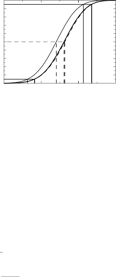
All this is illustrated in Figure 4.4, using the data above. In this graph we have also

reproduced, as the dashed curve, the conﬁdence function in Figure 4.3. Indicated is its median

value, which is the old estimate 0.66, together with the 90% conﬁdence interval (0.58, 0.74).

In addition there are two CDFs, both drawn as solid curves. The rightmost of these, which

is very close to the graph of the conﬁdence function, shows the a posteriori distribution for

p when we use the uninformative prior. We have also indicated its median value, together

with what would correspond to a 90% conﬁdence interval. However, in this setting, this

corresponds to a true probability statement – the probability that the value of p lies in this

108 THE ANATOMY OF A STATISTICAL TEST

0.1

0.2

0.3

0.4

0.5

0.6

0.7

0.8

0.9

Posterior probability CDF for p

0.5 0.6 0.7 0.8

Binomial proportion p

Figure 4.4 Bayesian analysis of a single binomial proportion. The solid curves are Bayesian

a posteriori distributions, the dashed curve is the frequentist’s conﬁdence function. The right

solid curve corresponds to the uninformed prior, the left one to an informed prior centered

on p = 0.4.

interval is 90%. The interval is therefore not called a conﬁdence interval, but a credibility

interval (both are conveniently abbreviated CI). Numerically we obtain the estimate 0.66

with 90% credibility interval (0.58, 0.74) – the same to two decimal places as found by

the frequentist.

The left solid curve in Figure 4.4 describes the a posteriori distribution when we use

the informed prior distribution above. Recall that the a priori distribution was centered

on p = 0.4, which is far to the left in this graph, so we see how the data have moved our

subjective assessment considerably toward larger values of p, and into a distribution for which

we have the median value 0.64 with 90% credibility interval (0.56, 0.71). This illustrates how

the Bayesian view of the world works: you update your collected knowledge when you get

new information.

Note the close agreement between the a posteriori distribution of p when using the un-

informed prior and the conﬁdence function. This is sometimes interpreted as implying that if

we have no prior opinion on p, we are almost in the frequentist situation. This is, however,

debatable. What is true is that in many situations you can ﬁnd a prior that is such that the

corresponding a posteriori distribution closely resembles the conﬁdence function. What is

debatable is whether it reﬂects ignorance: if we are ignorant about the value of p we are also

ignorant about the value of p

, but if p is uniformly distributed on (0, 1), then the CDF for p

would be F (x) =

√

x, which is not uninformative. However, things gets more bizarre, because

the CDF for the β(p; x + 1/2,n− x + 1/2) distribution actually improves the approximation

to the conﬁdence function. This case corresponds to taking as the a priori distribution the

β(1/2, 1/2) distribution, which (in this case) is called Jeffrey’s prior. Its probability den-

sity function is 1/

√

p(1 − p), which means that it puts very large weight on very small and

large values of p, and much less on intermediate values. So the best approximation to the

THE BELL-SHAPED ERROR DISTRIBUTION 109

conﬁdence function is not obtained by ignorance, but by putting weights on the boundaries.

In passing, we may note that this observation gives us what is actually a rather robust way to

obtain traditional conﬁdence intervals for p, by approximating the conﬁdence function with

this beta distribution. (We may also note that if Laplace had used this prior for his law of

succession, he would have found the odds to be 2n + 1 to 1 instead of n + 1to1asinthe

discussion above.)

4.7 The bell-shaped error distribution

The Italian priest and astronomer Guiseppe Piazzi discovered early in 1801 what he thought

was a new planet. He gave it the name Ceres, but after a while he lost sight of it when it

went behind the sun. There were so few observations made that astronomers were not able to

work out its orbit and therefore worried that they would not be able to locate it again, once

it emerged from behind the sun. Karl Friedrich Gauss, arguably the greatest mathematician

of all time, decided to give this problem his attention. After some lengthy calculations, he

predicted where Ceres would reappear. When it duly did so, Gauss’s fame spread far and

wide. At the time, Gauss did not communicate how he had arrived at his prediction, but it

later turned out that the method he used was what we today call the method of least squares.

Gauss had invented and used this method years earlier before he applied it to this particular

astronomical problem. He subsequently produced two proofs for the method. It is his ﬁrst

version that is of interest to us here, because it justiﬁes the choice of the Gaussian distribution

as a distribution for errors.

At the time it was customary in the natural sciences to use the arithmetic mean of repeated

observations, taken under essentially the same circumstances, as the estimate of the true value

of the phenomenon in questions. However, this method seemed not justiﬁed by the probability

distributions used at the time. Gauss ﬁlled this gap between statistical practice and statistical

theory by changing both the probability density and the method of estimation. With respect

to the former, the question was this: what does the error distribution look like, if the best way

to estimate the location is by taking the average? Using an argument, a modern short version

of which is given in Box 4.10, Gauss deduced that the distribution of the errors should have

a density which takes the form

ϕ(x) =



2π

−kx

for some constant k>0. Gauss pointed out that ‘the constant k can be considered as

the measure of precision of the observations’. He also made the comment that the dis-

tribution cannot truly represent a law of error, since it also assigns positive probabilities

to errors outside the range of possible errors; negative errors are often not possible and

there may be practical constraints on how large errors can be. Gauss considers this

feature unavoidable but of no importance because of the rapid vanishing of ϕ(x) for large

values of |x|.

This was, however, not the ﬁrst time the Gaussian distribution had appeared. In 1733

Abraham de Moivre derived it as an approximation to the probability that a binomial

variable is observed in a speciﬁed interval. His investigation was prompted by a need to

compute probabilities of winning in various games of chance, and what he demonstrated