Kallen A. Understanding Biostatistics

Подождите немного. Документ загружается.

150 EMPIRICAL DISTRIBUTION FUNCTIONS

0.1

0.2

0.3

0.4

0.5

0.6

0.7

0.8

0.9

Fraction of patients

6000500040003000200010000

sputumcount/gNeutrophil

0.2

0.4

0.6

0.8

6004002000

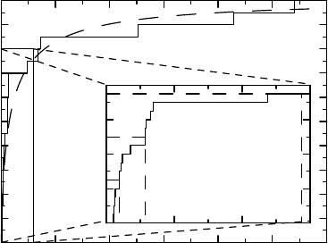
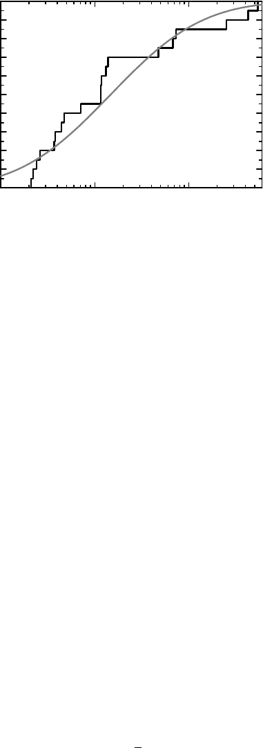
Figure 6.1 Illustration of data as an empirical distribution function. In the main graph,

the solid step function is the e-CDF and the dashed curve the population CDF. The inset

graph shows a blow-up of the initial part of the e-CDF, illustrating how some percentiles

are estimated.

all these x

. We now wish to look at the more general situation in which the outcome variable

can take on a multitude of different values, including the case where (in theory) it can take

on all possible values, at least in some interval. Well-known examples are blood pressure and

objective lung function measurements such as FEV

Consider the following 20 numbers: 37, 71, 24, 38, 44, 4286, 728, 26, 22, 138, 475, 47,

5408, 115, 131, 2520, 676, 21, 117, 115. They represent the neutrophil cell counts found in

sputum samples from 20 COPD patients. The medical meaning of this is not important, only the

assumption that these observations constitute a representative sample from some population.

We are going to use these data for illustrative purposes extensively in the upcoming discussion.

(The numbers are actually simulated, which explains why we can draw certain dashed curves

in some graphs below.)

One way to illustrate these 20 numbers graphically is the staircase function shown in

Figure 6.1. The data values are on the x-axis, at each of which there is a vertical step of

1/20, leading up to a monotonically increasing function starting at zero and ﬁnishing at one.

This function is called the empirical cumulative distribution function (e-CDF) of the data. We

usually denote it by F

(x), with n being the number of observations it is based on.

In the graph there is also a dashed curve. This represents another function, namely the

population CDF F (x), the distribution in the population of such data. This is what the e-CDF

(x) tries to estimate. The difference between the e-CDF and the CDF is that if we repeat

the experiment there will be a new e-CDF each time, although the CDF stays the same. This

means that F (x) is a characteristic of the outcome variable in the population (when measured

in the particular way of the speciﬁc protocol), whereas F

(x) is an estimate of F(x) from a

particular sample from that population. In general, statistics is divided into two main parts:

descriptive statistics which describes F

(x), and

inferential statistics which uses F

(x) to understand F (x).

HOW TO DESCRIBE THE DISTRIBUTION OF A SAMPLE 151

We have already noted that there are continuous and discrete stochastic variables. For

the former the CDF is a continuous function, whereas for the latter it is a step function.

Some data are hybrids of discrete and continuous data. For example, in order to assess a

person’s disability we may use a Visual Analogue Scale (VAS) which means that the disability

is described by a mark on a line going from 0 to 1, where 0 means no disability and 1 complete

disability. The corresponding CDF may have jumps at both the end points, but be a continuous

and increasing function in between.

The value of the e-CDF at the point x is the proportion of elements in the sample

,...,x

} that are at most x in magnitude. It therefore has the analytical expression

(x) =



i=1

I(x

≤ x), (6.1)

where I(C) denotes the indicator function which is 1 if the condition C is true and 0 if it is false.

If precisely k of these x

are less than or equal to a particular value x, then F

(x) = k/n.Ifso,

and x is one of the observations, we call k the rank of x and denote it by R

(x) (which therefore

is equal to nF

(x)). (If there are ties, a modiﬁcation is needed.) There is a fundamental theorem

in probability theory, called the Glivenko–Cantelli theorem, which says that the e-CDF F

(x)

converges to F (x) (in a uniform way in x), as the sample size n increases.

The e-CDF is deﬁned as a (right-continuous) step function. For many purposes it would

have been more convenient, at least for a continuous CDF, to deﬁne it as a piecewise linear

function such that the point (x

,F(x

)) is connected to (x

k+1

,F(x

k+1

)) by a straight line,

instead of via the point (x

k+1

,F(x

)) (the staircase). We will, however, mostly stick with

the convention, except for a few occasions when we point out some beneﬁts of the linearly

interpolated version, when this clariﬁes a particular statistical method.

There is an alternative formula for the e-CDF. Its derivation is based on the observation that

for any monotone function we have that F (x) = F (x−) + F (x), where F(x) is the jump at

the point x and F (x−) is the left-hand limit of F (x). If we rewrite this for the complementary

function F

(x) = 1 − F (x), we get

(x) = F

(x−) − F (x) = F

(x−)



1 −

F (x)

(x−)



This is an observation which only is of interest at jump points, and since the e-CDF consists

exclusively of jump points, it is particularly useful for that function. In fact, if we apply the

observation repeatedly to the e-CDF, we get the alternative formula for F

(x), referred to

above. The way it is computed is as follows. Order the different values in the sample into a

strictly increasing sequence x

<...and let d

denote the number of observations with

value x

. Let r

= nF

−) be the number of observations that are at least x

in size. The

formula then reads

(x) =



j;x

≤x



1 −



where



means that we should multiply all the a

that fulﬁll the criterion deﬁned in C.

This way of writing the e-CDF is called the Kaplan–Meier form of the e-CDF, or the Kaplan–

Meier estimate of the CDF. It has the important property that it can be generalized to some

situations where there is incomplete knowledge in the data. If we study the time until some

152 EMPIRICAL DISTRIBUTION FUNCTIONS

particular event occurs, this event may not occur for some patients during the observation

period, in which case we only know that the true observation is larger than the observation

time. In such a case we can use the Kaplan–Meier form of the e-CDF to estimate F (x), which

is useful in the analysis of survival data.

The discussion above applies equally well to continuous and discrete CDFs, but there

are some aspects of the latter that should be emphasized. To be able to plot the e-CDF for a

discrete distribution, we need the observations to be ordered. For a binomial, for example, we

can code no event as x = 0, and event as x = 1. An observation k from a Bin(n, p) distribution

is then the sum of n independent observations of a Bin(1,p) distribution, which is such that

the CDF has jump 1 − p at x = 0, followed by another jump of size p in the point x = 1.

The e-CDF is the corresponding jump function, for which the jump at x = 0is1−k/n and

at x = 1isk/n. This can be generalized to data that fall into more than two categories, as

long as these are ordered so that we actually can draw the graph of the CDF F (x). If so, it is

no restriction to code the categories as k = 1,...,c. We may, for example, assign a disability

index in c categories to patients who have had a stroke, which represents a judgement of how

disabled they are, in such a way that a larger score means that the patient is more disabled.

Such data are simply described by the probabilities p

of falling into each category j, and

we have that the CDF is a cumulative sum of these p

, that is, F (k) = p

+ ...+ p

. This

deﬁnes a step function, an example of which is shown in gray in Figure 6.2. In this case the

jump points of the CDF and the e-CDF of a particular experiment will coincide, though the

actual jump sizes may differ.

Ordered categorical data can often be perceived to be a discrete approximation of some

underlying continuous variable. For the disability score above we may assume the existence of

a continuous (and probably unmeasurable) disability variable X with a continuous CDF F (x),

together with a series of cut-off points a

=−∞<a

<...<a

c−1

=+∞, such that

our ordered categorical variable takes the value k precisely if a

k−1

<X≤ a

. The probability

of falling into category k is then given by p

= F(a

) − F (a

k−1

We have pointed out that some aspects of statistics would have been conceptually simpler

with the e-CDF deﬁned by linear interpolation. This applies to the CDF of a discrete distri-

bution as well, in that it is not clear why the CDF should be right- and not left-continuous

0.1

0.2

0.3

0.4

0.5

0.6

0.7

0.8

0.9

876543210

disabilityofDegree

Figure 6.2 Illustration of how we can consider ordinal data derived from an underlying

continuous distribution, with cut-off points 2 < 3.5 < 4.5 < 6.

DESCRIBING THE SAMPLE: DESCRIPTIVE STATISTICS 153

0.1

0.2

0.3

0.4

0.5

0.6

0.7

0.8

0.9

0.5

− p

Δ F(1)

Δ F(0)

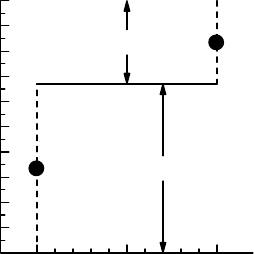
Figure 6.3 The mid-point CDF for a two-point distribution.

at jump points. What corresponds to linear interpolation in such a case would be to take the

mid-value of the jump as the deﬁnition of the CDF at that point. This provides the same

staircase function as the traditional one, except for the values at the actual jumps. If F (x)is

the traditional, right-continuous, distribution, then we redeﬁne the CDF to take the average

value (F(x−) + F(x))/2 at the point x. This is illustrated for a two-point Bin(1,p) distribution

in Figure 6.3. We will later see the usefulness of this modiﬁed CDF in connection with the

Wilcoxon test for discrete data. We should also note that this is precisely the mid-P adjustment

mentioned in equation (4.2), where we constructed the conﬁdence function for a parameter

in a discrete distribution.

If we have c ordered categories, labeled 1,...,c, then the jumps p

= F(k) are prob-

abilities, and the CDF is that of the multinomial, Mult

(1,p

,...,p

), distribution. If we

perform n experiments resulting in observed frequencies x

,...,x

, the e-CDF is the step

function with jump x

/n at the point k. Moreover, there are only ﬁnitely many possible out-

comes of a multinomial distribution, so there are a ﬁnite number of possible e-CDFs, namely



n+c−1



. This has implications for how p-values can be computed.

6.3 Describing the sample: descriptive statistics

We will now see how we can describe the e-CDF of a sample {x

,...,x

} using various

summary statistics. Though the most complete way to describe the sample is to list it (not

practical unless the sample is small) or plot it, there is often a need to summarize its key

aspects in some convenient and easily communicable way.

One way to do this is to choose some value between 0 and 1 and describe where the

e-CDF is equal to this particular value. In other words, choose 0 <p<1 and solve the

equation F

(x) = p for x = x

. Because F

(x) is a step function this cannot always be done

exactly, and we may need to average two numbers. As an example, take p = 0.5. This means

that we want the value x

0.5

for which half of the observations are less than or equal to it. If n

is odd, x

0.5

is obtained by ordering the sample and take the middle number. If n is even, we

need to take a number between the two values that are in the middle of the sample, and by

convention we take the arithmetic mean of these. We call x

0.5

the median of the sample. (This

is one instance when using linear interpolation to deﬁne the e-CDF would help: it would deﬁne

154 EMPIRICAL DISTRIBUTION FUNCTIONS

0.1

0.2

0.3

0.4

0.5

0.6

0.7

0.8

0.9

Fraction of patients

9876543210

Value of outcome

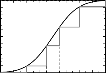
Figure 6.4 Approximating an empirical distribution function, which describes a large data

set, by a piecewise linear function deﬁned by percentiles.

a unique sample median, providing a better estimate of the median of the true distribution.)

The general x

is called a percentile, and as for x

0.5

we have special names for x

0.25

and x

0.75

the lower and upper quartiles. By describing a set of percentiles and adding the smallest and

largest observations, we get a smaller set of data, which can be used to obtain an approximation

of the e-CDF. This is illustrated in Figure 6.4, where the e-CDF of a sample of 200 points from

a continuous distribution is approximated by the 10th and 90th percentiles, the quartiles and

the median: a stepwise linear function connecting the smallest and the largest observations

with break points at these percentiles may be a fairly good approximation to the CDF.

It should be noted that what value a percentile assumes does not depend on all the individual

observations in the sample. Take the median as an example. Its value is the value in the middle

of the sorted sample, but does not depend on the exact values of those data points that are less

than (or larger than) this value, except that they are smaller (or larger).

The most popular way of summarizing a data set is through the (arithmetic) mean

¯x =



i=1

together with the standard deviation s, which is the square root of the sample variance

n − 1



i=1

− ¯x)

The mean is a measure of the location of data and the standard deviation is a measure of the

dispersion around the mean. These sample parameters estimate the corresponding population

parameters (which were deﬁned in Box 4.5 and will be revisited in the next section).

However, ¯x and s are not always good measures for describing the CDF. For the sputum

data shown in Figure 6.1 the mean is 752.0 and the standard deviation is 1521.1. Compare

this with the three quartiles 37.5, 115.0, 575.5, shown in the small subplot in Figure 6.1. We

see that the upper quartile, below which 75% of the data lie, is much smaller than the mean.

DESCRIBING THE SAMPLE: DESCRIPTIVE STATISTICS 155

Box 6.1 The lognormal distributions

If the logarithm of a stochastic variable X has a Gaussian distribution, ln X ∈ N(m, σ

we say that X has a lognormal distribution. Its CDF is given by F (x) = ((ln x − m)/σ),

from which some calculus shows that its mean and variance are given by

E(X) = e

m+σ

and V(X) = e

2m+σ

− 1),

respectively. The median is e

, which we can derive from the general observation that

for a monotonic transformation h(x) we have that

median(h(X)) = h(median(X)),

here applied to h(x) = e

. The same applies to any other percentile. The coefﬁcient of

variation is by deﬁnition CV =

√

V (X)/E(X), and is a dimensionless expression of

variability. For the particular case of the lognormal distribution we ﬁnd that

CV =



− 1.

Note that for σ

small we have that CV ≈ σ =

√

V (ln X).

The reason for this is obvious from the formulas above in combination with Figure 6.1; the

distribution is skewed to the right in the sense that most of the data is concentrated in the left

portion of the graph, but with a long tail of large values to the right. In such a case the choice

of mean and standard deviation as descriptors of the e-CDF, and ultimately the CDF, may be

rather poor and misleading. Implicit in the choice of these sample statistics as descriptors of

the e-CDF lies an assumption that the distribution is reasonably symmetric around its mean.

When the distribution is symmetric around its mean, the median should be equal to it, so

if the difference between these two parameters is large, the distribution is skewed. (This is

not to say that you do not want to estimate the mean for a skew distribution, only that more

information is needed to understand the CDF.)

When a distribution is skewed to the right, and the data are positive, we may try to

symmetrize it by taking the logarithms of the data. This means that we replot the e-CDF

on a logarithmic scale, as we have done in Figure 6.5 for the sputum data. The mean

in this graph corresponds to the geometric mean 147.2 of the original data. More pre-

cisely, this is the arithmetic mean of the logarithmic data, rescaled to the original scale

by exponentiation:

ln x





i=1



1/n

This number is much closer to the sample median, which we saw above was 115, and is in

this case a meaningful description of the center of the distribution. To describe the variability

for a lognormal distribution we can use the coefﬁcient of variation for that distribution,

CV =



− 1 (see Box 6.1), where s

is the sample variance of ln x

. Multiply it by 100,

and we express the coefﬁcient of variation as a percentage. For our sputum data it is 469%.

156 EMPIRICAL DISTRIBUTION FUNCTIONS

0.1

0.2

0.3

0.4

0.5

0.6

0.7

0.8

0.9

Fraction of patients

Neutrophil count/

sputum

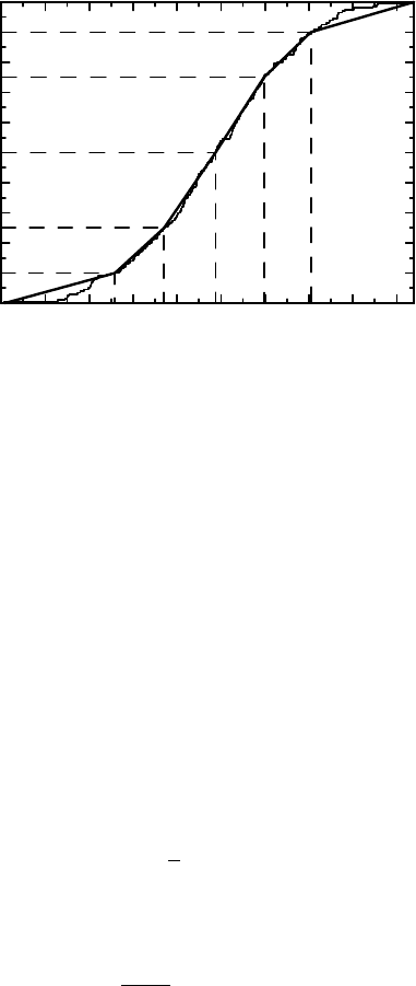
Figure 6.5 Illustrating sputum data as an empirical distribution function with a logarithmic

scale. The gray curve is the reconstructed CDF from the observed mean and standard deviation

of the logged data.

When we discussed percentiles, we emphasized their ability to reconstruct the e-CDF.

How can we reconstruct the e-CDF from the mean and standard deviation? This is done based

on the Gaussian distribution in such a way that we reconstruct F (x)as((x − ¯x)/s). The

dashed curve in Figure 6.5 shows this for the sputum data, albeit on a logarithmic scale.

We see that the mean and standard deviation of the logged data (or the geometric mean and

coefﬁcient of variation on the original scale) represent a reasonable summary of these data.

6.4 Population distribution parameters

Descriptive statistics have their counterpart for the population CDF F (x). To describe this

we use the notation that was introduced in Box 4.8, but we repeat it here because of the

fundamental role it will play in our discussion from now onwards. The notation is that we

write dF (x) = f (x)dx for a point x where a particular distribution is (absolutely) continuous,

and dF (x) = F(x) for a point x where there is a jump of size F (x). Based on this, we

denote sums and integrals by use of the common notation



g(x)dF (x).

If F (x) is piecewise differentiable with derivative f (x), this is



g(x)dF (x) =



g(x)f (x)dx,

whereas for a e-CDF F

(x), computed from the data {x

,...,x

}, it becomes



g(x)dF

(x) =



i=1

g(x

POPULATION DISTRIBUTION PARAMETERS 157

since dF

) = 1/n in this case. When F(x) is a population CDF the integral represents the

average of the values g(x) in the whole population and is therefore a population parameter.

It is estimated by replacing F (x) with the e-CDF F

(x) in the computation, deﬁning the

sample parameter.

As a ﬁrst example, recall that the mean of F (x) is deﬁned as

m =



∞

−∞

xdF(x).

To estimate it, we replace F (x) with F

(x) and get the sample mean:

¯x =



∞

−∞

xdF

(x) =



The mean is obviously a location measure, being the average of all values. To describe it

geometrically, we can rewrite it as

m =



∞

(1 − F (x))dx −



−∞

F (x)dx.

This means that we can interpret the mean as the area between the curve y = F (x) and the line

y = 1 for positive x, minus the area under the curve y = F (x) above the x-axis for negative x.

More importantly, the formula gives us a way to visualize the difference in the mean values

for two distributions. In such a case, if m

is the mean for the CDF F (x) and m

that for

G(x), then

− m



∞

−∞

(G(x) − F (x))dx,

which is the area enclosed by the CDFs.

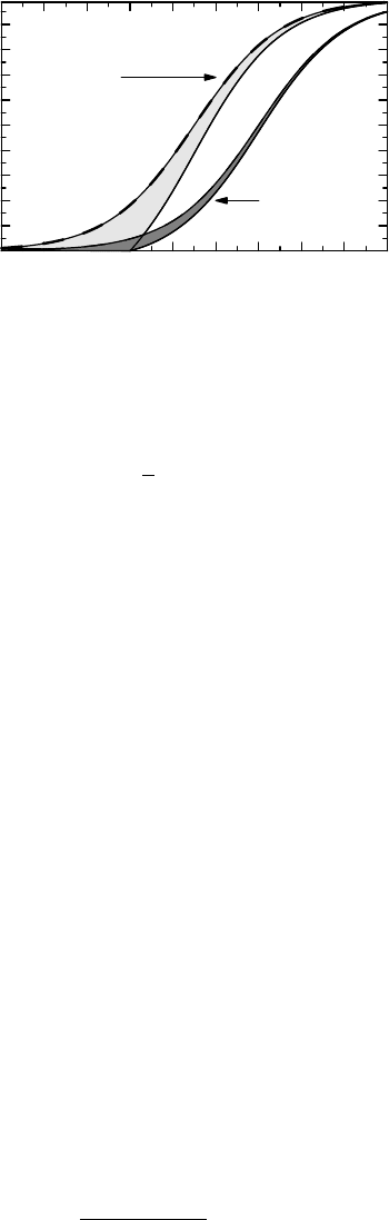
Example 6.1 As an example, consider Figure 6.6, which is a reproduction of the graph that

illustrated the effect of differential drop-out in Section 3.7. The area between the dashed and

solid curves for a group shows the effect that missing data have on the mean value in that

group. Inspecting the graph, we see that the area between the two solid curves is smaller than

the area between the two dashed curves, showing that, if we analyze completers only, we get

a bias toward no effect in the mean.

We can also visually estimate the bias with the LOCF approach. This would mean that we

impute the value −1 for missing data, which means that the distribution for LOCF imputed

data is zero up to the point x =−1, where there is a jump up to the dashed curve. The area

between these two CDFs is the area between the dashed curves over the region x>1. The area

between the curves to the left of x =−1 is therefore the bias we get by the LOCF approach.

Comparing areas, we see that in this case LOCF is less biased than analyzing completers only.

To measure the spread, or dispersion, of the distribution, a common measure is the popu-

lation variance deﬁned by



∞

−∞

(x − m)

dF (x). (6.2)

158 EMPIRICAL DISTRIBUTION FUNCTIONS

0.1

0.2

0.3

0.4

0.5

0.6

0.7

0.8

0.9

Proportion of patients

−4 −3 −2 −1 543210

Chan

e from baseline

Placebo

Active drug

Figure 6.6 Reproduction of Figure 3.1, illustrating how we can assess the effect on the mean

by comparing areas.

If we replace F (x) with F

(x), we see that this should be estimated by

(m) =



− m)

However, this only works if we know the mean m. If we do not, we need to estimate it with the

sample mean and use

(¯x) as the estimate of σ

. For this to be an unbiased estimator we need

to replace the denominator n with n − 1, which gives us the sample variance s

. Intuitively the

reason is that though we have n terms, there are only n − 1 independent ones, since subtracting

¯x means that the sum of the terms x

− ¯x is constrained to be zero. By analogy, with more

parameters, say p, to estimate, we would in general have to divide by n − p. There are ways

to derive the correct denominator directly by eliminating the mean from the problem. One

way uses the differences x

− x

and is outlined in Box 8.6, another is based on the residuals

− ¯x and the likelihood theory for Gaussian data and is discussed in Box 13.1. For both of

these derivations the situation is complicated by the fact that the data analyzed are dependent.

It is interesting to note that the bias adjustment of the variance made by dividing by n − 1

instead of by n is not usually done when we estimate proportions in a binomial distribution.

The variance estimator for the frequency ˆp is usually taken to be ˆp(1 − ˆp)/n, which is biased

for the reason above; the unbiased estimator is ˆp(1 − ˆp)/(n − 1).

The mean is a measure of location, and so are the percentiles, which are deﬁned for the

population CDF in the same way as the sample percentiles were deﬁned for the e-CDF – as the

solution of the equation F(x) = p. This deﬁnes the population percentiles which we estimate

by the sample percentiles, as discussed in the previous section.

6.5 Conﬁdence in the CDF and its parameters

Foragivenx, the value F (x) of the CDF is a probability and the value of the e-CDF F

(x)

is an observed relative frequency, such that nF

(x) follows a Bin(n, F(x)) distribution. Since

V (F

(x)) = p(1 − p)/n, this means that the set of ps that satisfy



n(F

(x) − p)

p(1 − p)



≤ 1 − α

CONFIDENCE IN THE CDF AND ITS PARAMETERS 159

0.1

0.2

0.3

0.4

0.5

0.6

0.7

0.8

0.9

Fraction of patients

Neutrophil count/

sputum

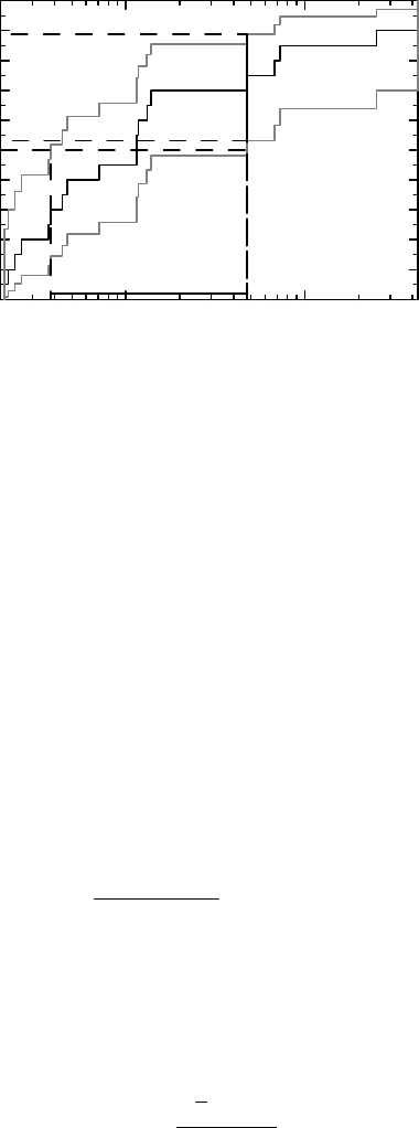
Figure 6.7 Illustration of how to obtain conﬁdence limits for percentiles, using pointwise

conﬁdence limits for the CDF.

constitute a conﬁdence interval for F (x) of degree 1 − α. Figure 6.7 illustrates this for the

sputum data. The black step function is the original e-CDF, and the two solid gray step

functions above and below it deﬁne (the end points of) the 95% conﬁdence limits. One such

conﬁdence interval is also illustrated as the thick vertical line above the point x = 475. It

is important to point out that these intervals are pointwise conﬁdence intervals: to get the

correct conﬁdence degree we ﬁrst need to ﬁx the point x. If we do not prespecify the point

x, we have a multiplicity problem. The natural follow-up question is then to ask for limits

that by construction contain the complete CDF F (x) with 95% probability. Such a region

is made up of simultaneous conﬁdence intervals, and its construction is brieﬂy addressed in

Appendix 6.A.2.

In Figure 6.7 we also have a horizontal line which is deﬁned from the gray conﬁdence limit

curves at level 0.5. The interval it deﬁnes has limits 38 and 475. These are (approximate) 95%

conﬁdence limits for the median of F (x). Conﬁdence limits for other percentiles are obtained

in the same way. The argument is the following simple observation: ﬁnding the conﬁdence

interval for a parameter θ such that F (θ) = p is the same as ﬁnding all θ such that



n(F

(θ) − p)

p(1 − p)



≤ 1 − α

(the same as above, except that now p is held ﬁxed).

To obtain conﬁdence intervals for the mean is done in an altogether different way, which is

not easily described in geometric terms. The computation is based on the fact that ¯x (according

to the CLT) asymptotically has a Gaussian distribution with mean m and variance σ

/n, where

is the variance of F (x). This suggests the use of the conﬁdence function

C(m) = 



√

n(m − ¯x)



which should be at least approximately valid for learning about the mean m. The problem

here is that we do not know σ

, a problem we solve by estimating it by the sample variance s