Kallen A. Understanding Biostatistics

Подождите немного. Документ загружается.

160 EMPIRICAL DISTRIBUTION FUNCTIONS

This means that the (approximate) symmetric conﬁdence interval, of conﬁdence degree 1 − α,

for the mean is computed from the well-known formula



¯x − z

α/2

√

, ¯x + z

α/2

√



However, whether this approximation is good or not depends on how skewed (i.e., non-

symmetrical) the distribution F(x) is (and how heavy the tails are). If n is taken sufﬁciently

large, it can be made as good as we want, but it may require very large values of n.Onthe

other hand, when F (x) is very symmetric around the mean, a relatively small n might sufﬁce.

The extreme case here is when F (x) is in fact Gaussian in itself, in which case the conﬁdence

function C(m) is exact if σ

is known. If σ

is not known, but needs to be estimated by s

the mathematical analysis has been taken one step further, to obtain an explicit, analytical,

description of the true distribution of

√

n(¯x − m)/s. This is the t distribution with n − 1 degrees

of freedom, which we denote t(n − 1) (a derivation of this is outlined in Appendix 6.A.1).

So, if we let T

(x) denote the CDF of the t(n) distribution, we have in this case the exact

conﬁdence function

C(m) = T

n−1



√

n(m − ¯x)



The corresponding conﬁdence interval is wider than that for the normal approximation; how

much wider depends on the size of n. The following example illustrates this.

Example 6.2 To illustrate the conﬁdence functions for the mean we use the data that Student,

the inventor of the t distribution, used for illustration. These data are often referred to as the

Cushny and Peebles data and consist of the following list of paired observations from 10 sub-

jects: (0.7, 1.9), (−1.6, 0.8), (−0.2, 1.1), (−1.2, 0 .1), (−0.1, −0.1), (3.4, 4.4), (3.7, 5.5),

(0.8, 1.6), (0.0, 4.6), (2.0, 3.4). In this example we analyze the data obtained by computing

the difference for each pair. Figure 6.8 contains two conﬁdence functions for this data set,

the conventional t-test and the large-sample approximation which uses the Gaussian CDF

(x). We see that ignoring the extra variability that led to the deﬁnition of the t distribution

will produce shorter conﬁdence intervals than the correct one, as expected.

Recalling how we obtained conﬁdence intervals for a binomial proportion in Section 4.6.1,

it may be natural to ask if we should not use the ratio

√

n(m − ¯x)/

(m) as a test statistic

instead. At ﬁrst glance it may appear that this should have a t(n) distribution, but it does

not, because the numerator and denominator are now dependent. Its distribution is given in

Appendix 6.A.1, where it is shown that the conﬁdence function for m it deﬁnes is equivalent

to the t(n − 1)-based conﬁdence function above.

As outlined in Box 6.2, the t-based conﬁdence function also has a Bayesian interpretation:

if we assume very special prior distributions for m and σ, the function C(m)isthea posteriori

distribution for m. However, for this we need to use rather peculiar prior distributions for m

and σ, at least from a probabilistic point of view.

CONFIDENCE IN THE CDF AND ITS PARAMETERS 161

Box 6.2 Bayesian approach to a Gaussian distribution

Given independent observations x

,...,x

from a N(m, σ

) distribution, the sample is

an observation of a distribution with probability density



i=1



− m



(2πσ

)

n/2

exp



−



− m)

2σ



= (2πσ)

−n

exp(−Q/2σ

where

Q = (n − 1)s

+ n(¯x − m)

= (n − 1)



1 +

n − 1



,t=

m − ¯x

√

If we assume that the prior distributions for m and σ

are independent, and that the

prior for σ

corresponds to the measure dσ

/σ

(which is not a probability measure,

but means that the precision variable σ

−2

has a uniform distribution), we can obtain the

marginal distribution for m by ﬁrst integrating σ

out, and then multiply by the prior

for m. To integrate, we introduce the new variable y = 1/σ

, and get the integral

(2π)

−n/2



∞

n/2−1

exp(−Qy/2)dy ∝ Q

−n/2

This means that the density for m is proportional to (1 + t

/(n − 1))

−n/2

, which de-

ﬁnes the t(n − 1) distribution. If we therefore take the uninformative prior dm for m,

we see that the posterior density for m, given the observed data, is derived from the

observation that

m − ¯x

√

∈ t(n − 1).

If we have some prior information on m (but none on σ

) we simply multiply the t(n − 1)

density with this a priori density and normalize, to obtain the a posteriori distribution.

0.1

0.2

0.3

0.4

0.5

0.6

0.7

0.8

0.9

Confidence in m

Mean m

t(n − 1)

N (0, 1)

Figure 6.8 Conﬁdence functions describing our information about the mean. The solid black

curve corresponds to Student’s t-test, the gray curve to the Gaussian approximation.

162 EMPIRICAL DISTRIBUTION FUNCTIONS

6.6 Analysis of paired data

We next return to the COPD patients and their sputum data, but now we assume we have

two observations on each of the 20 subjects. The second set of data consists of the following

numbers (paired with the previous sequence): 18, 19, 2, 2, 5, 515, 30, 10, 3, 55, 127, 2, 260,

16, 8, 301, 443, 1, 26, 24. The original observations (X) were taken after some drug was

given, whereas the new data (Y ) were obtained under the same conditions, but without this

drug. Precisely as with Cushny and Peebles data in the previous section, we wish to analyze

the difference Z = Y − X. Our intention here is to have a more general discussion about what

we can do by exploring the CDF for Z, noting that if X and Y have the same distribution,

the distribution for Z would be symmetric around zero (see equation (4.1)). We wish to ﬁnd

ways to explore this symmetry in order to obtain a test for the null hypothesis that there is no

effect of the drug.

The immediate consequence of the symmetry is that both the median and the mean of Z are

zero. One way to test the null hypothesis is therefore to test if either of these two parameters

are zero. For the mean we get the estimate −659 with 95% conﬁdence limits (−1318, 1), and

for the median we get the estimate −87 with 95% conﬁdence limits (−235, −39). For the

mean there is not sufﬁcient evidence to reject the null hypothesis at the conventional two-sided

5% level, since the interval contains zero, whereas based on the median we have sufﬁcient

evidence. However, because of the skewness of the data, the proposed conﬁdence interval for

the mean may be quite inaccurate (have the wrong error control). We will see that this is the

case in the next section.

The mean and median estimates are quite different, and from our previous discussion we

have a fairly good idea of why this is: we should probably log our data before we analyze. The

analysis should therefore be on the stochastic variable Z = ln Y − ln X = ln(Y/X) instead.

The mean and median of this distribution should then be back-transformed to the original

measurement scale by exponentiation. As discussed earlier, when we exponentiate the (arith-

metic) mean of the logged data, we get the geometric mean of the original data, whereas when

we exponentiate the median of the logged data, we get the median of the original data. For

our data the geometric mean estimate is 0.14 with 95% conﬁdence limits (0.09, 0.21), and

for the median the estimate is 0.13 with 95% conﬁdence limits (0.06, 0.22). We see that we

get more consistent results by analyzing logged data instead of the original data, but the ﬁnal

claim is different: the ﬁrst is the ratio of the geometric means obtained with and without drug

treatment, and the second is the median of the individual ratios.

What if we analyze the ratio Y/X directly? The median is the same, but now the mean is

the arithmetic mean of the ratio, estimated as 0.19 with 95% conﬁdence limits (0.12, 0.27).

This is not the ratio of the individual means (as is true for the geometric mean) and may

therefore not be a natural measure of the location of the data. If we want to discuss a mean

ratio we should analyze differences of logged data instead (see Box 6.3).

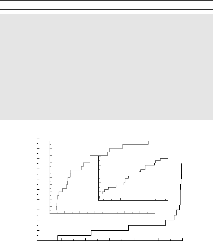
In Figure 6.9 we have plotted the various e-CDFs discussed above. The largest, outer, graph

shows the e-CDF for the difference, which is highly skewed to the left, making measures like

the mean more or less meaningless. The middle graph shows the e-CDF for the ratios on the

original (linear) scale. This is also slightly skewed, but now to the right. Finally, the innermost

graph shows the same e-CDF but now on a logarithmic scale. This is the most symmetric of

the e-CDFs, and the scale we should work on for these data (supported by the fact that when

we consider cell counts in sputum, it is the relative effect that has clinical meaning).

BOOTSTRAPPING 163

Box 6.3 When should we log the data in the analysis?

This question is an important one that does not have a simple, deﬁnite answer. But there

are a few points to be considered.

One situation in which to consider log-transformation is when we have a skewed distri-

bution with a long tail to the right. Log-transformation may or may not symmetrize the

distribution in this case; if it does there is still the problem of justifying why we should

describe this variable in this way.

To me the main driver behind the choice to log-transform the data is how the experienced

clinician, or scientist, sees the variable in question. Does he think of effects as absolute

changes, or as relative changes? If the answer is absolute changes, the choice should

be to analyze the data on the original scale. If, on the other hand, the answer is relative

changes, that means interpreting effects in a relative sense, so that the expression dE/E

represents the true effect. In such a case the analysis should be done on ln E. There

are no other changes to how we set up the model, but care must be taken with the

description of the end result. Usually a mean difference on the logarithmic scale should

be back-transformed to a ratio of (geometric) means.

0.1

0.2

0.3

0.4

0.5

0.6

0.7

0.8

0.9

−6000 −5000 −4000 −3000 −2000 −1000 0

Y − X

0.1

0.2

0.3

0.4

0.5

0.6

0.7

0.8

0.9

0.10 0.2 0.3 0.4 0.5 0.6 0.7

Y/X

0.2

0.4

0.6

0.8

−1

Y/X

Figure 6.9 The e-CDFs for Y − X and Y/X, the latter on both a linear and a

logarithmic scale.

6.7 Bootstrapping

We have discussed how we can describe a population CDF F (x) in terms of various (popu-

lation) parameters, and how these can be estimated from a random sample. The tricky part

164 EMPIRICAL DISTRIBUTION FUNCTIONS

is to describe the actual knowledge we obtain about the parameter from our estimate, that is,

how close we believe it is to the true value. We have outlined how we can do this in special

situations, such as for percentiles and the mean. However, there may be other parameters we

wish to estimate, and it may not be trivial to derive conﬁdence statements for these. In such

situations a method of considerable conceptual simplicity comes to the rescue, but it is rather

computer-intensive (though this is less of a problem now than it used to be).

To specify the problem, from a particular random sample {x

,...,x

}we wish to compute

a particular function

θ(x

,...,x

), often an estimator of a parameter θ. We can compute the

estimate, but how do we get conﬁdence statements about θ? We have seen how such statements

can be obtained for percentiles by using the e-CDF F

(x) together with knowledge about the

binomial distribution. The mean, in turn, used a different method which did not work well for

the sputum data on the original scale, because the distribution was so skew. How can we get

more reliable conﬁdence statements for the mean on the original scale?

To understand the method to be described, we ﬁrst note that if we knew the true CDF F (x),

we could obtain such information with any prespeciﬁed precision by employing an in silico

experiment. We do this by obtaining the distribution of

θ (which is a function of a sample) by

constructing a very large number of independent samples from the distribution, computing the

test statistic for each of these and investigating the distribution of these computed numbers.

A single such simulation is how the collection of data from one experiment works, and we

can do this on the computer as many times as we wish. The fact that we do not know F (x)

poses a problem, but we have data from an experiment, and with it an approximation of F (x)

as the linearly interpolated version of the e-CDFs (instead of the step function version; see

page 151). We therefore start this discussion by assuming that F

(x) is a linearly interpolated

e-CDF, and that this function is a good description of the true (but unknown) CDF F (x). We

then generate new random samples using the following process:

1. Choose n random numbers p

from the uniform distribution on the unit interval.

2. For each of these, compute the percentiles x

= F

−1

3. Compute the function

θ(x

,...,x

On the computer we can do this as many times as we wish. This will produce a random

sample {θ

,...,θ

} of function values, which can be used to describe the distribution of

θ.

The process therefore deﬁnes an approximation to the conﬁdence function for θ, from which

we can compute any (approximate) conﬁdence interval or p-value we wish. How well this

works obviously depends on how well F

(x) approximates F (x), but it is expected to improve

as we increase the sample.

As already hinted, this is not the method we actually use, because the e-CDF is not deﬁned

by linear interpolation, but as a staircase function. If we repeat the procedure described above,

we now get our simulated data values only among the original observations. If these are all

different, we can get for each random number any of these with equal probability; if there are

ties such numbers will turn up proportionally more often. But this means that the procedure

above is the same as taking a random sample from the original data set by sampling with

replacement. This deﬁnes the bootstrap method and for clarity we repeat how it works.

1. Generate a large number N of samples by sampling with replacement from the data

,...,x

BOOTSTRAPPING 165

2. For each sample i, compute the function value as θ

3. Use the (linearly interpolated) e-CDF for the data {θ

,...,θ

} as a conﬁdence function

for θ.

The term ‘bootstrapping’ was introduced by Bradley Efron and is taken from the phrase ‘to

pull oneself up one’s bootstrap’, from the famous Adventures of Baron Munchausen, where

in one story the baron used this method to escape from the bottom of a deep lake.

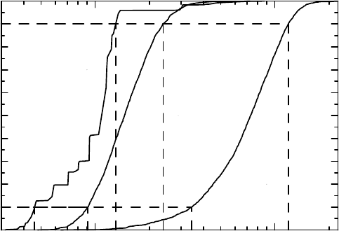
Example 6.3 To illustrate bootstrapping, consider our original sputum cell count data. Using

2000 samples, the process mentioned above gives us the conﬁdence curves in Figure 6.10 for

the median, the geometric mean and the arithmetic mean. Note that the data have been analyzed

on the original scale, but we display them on a logarithmic scale for presentational clarity.

The graph also illustrates the corresponding symmetric 80% conﬁdence intervals for each of

these parameters.

We can use this approach for any parameter we wish, including the value of the CDF

F (x) itself at a given point x. We can also provide estimates with conﬁdence intervals

for some more unconventional parameters in the same way. We can look at the difference

of the mean and the median to demonstrate that the distribution is not symmetric, or we

may use the difference between the median and the average of the two quartiles for the

same purpose.

If we apply this to the comparison of the two stochastic variables Y and X we dis-

cussed in the previous section, we can compare those results with the results obtained

using bootstrapping.

0.1

0.2

0.3

0.4

0.5

0.6

0.7

0.8

0.9

valueparameter

median

meangeometric

meanarithmetic

Figure 6.10 Bootstrapped conﬁdence curves for statistics of the sputum count data

(obtained on the original scale, but shown on the log scale), demonstrating how we obtain

their conﬁdence limits.

166 EMPIRICAL DISTRIBUTION FUNCTIONS

Example 6.4 The table below compares what we get using the bootstrap method (Boot), in a

run with 2000 samples, with the results we derived in the previous section (NP), for the median

and the mean. We make the comparison both for the difference, labeled Y −X, and for the

difference of the logged data, labeled Y/X. What is shown are estimates and 95% conﬁdence

limits. For the bootstrap samples the point estimate is the median of the conﬁdence curve.

Analysis of Y − X Analysis of Y/X

Median Mean Median Mean

NP Boot NP Boot NP Boot NP Boot

Lower CL −235 −208 −1318 −1360 0.09 0.09 0.06 0.07

Estimate −87 −87 −659 −650 0.14 0.14 0.13 0.13

Upper CL −39 −38 1 −126 0.21 0.20 0.22 0.24

We ﬁnd consistency in the results for the two methods when it comes to the analysis of the

ratio, and also when it comes to the analysis of the median for the difference. However,

the upper limit for the mean has been lowered considerably now, which justiﬁes our earlier

cautionary remark about the NP conﬁdence interval for the mean with skewed data.

6.8 Meta-analysis and heterogeneity

It may be tempting to view meta-analysis in roughly the same way as we view the bootstrap

method: you have a number of different estimates of a parameter in a series of studies, so why

not apply the bootstrap idea to obtain the pooled information by looking at the CDF generated

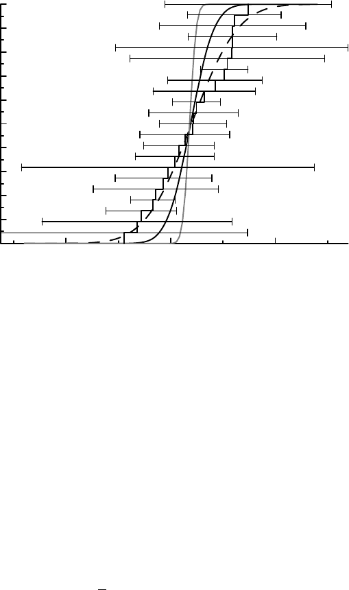
from the individual study results? As an example, consider a meta-analysis carried out in the

mid 1980s on 22 clinical trials, each of which investigated whether the use of beta-blockers re-

duces mortality after a heart attack. The 22 odds ratios (treated versus control) for the individual

trials are shown in Figure 6.11 as an e-CDF versus logged odds ratio (the staircase curve).

Before we discuss the graph in detail, we perform the conventional Mantel–Haenszel

analysis (see Section 5.5) on these data. Such an analysis gives us an estimated pooled odds

ratio of 1.20 with 90% conﬁdence interval (1.10, 1.30). The traditional analysis also includes

a test for homogeneity, the Breslow–Day test, with p-value 0.063, which is close to being

statistically signiﬁcant at the conventional 5% level. This would be the standard output of a

conventional meta-analysis for these data. On the log scale the odds ratio and 90% conﬁdence

interval are given by 0.18 and (0.10, 0.26), respectively.

As already mentioned, the e-CDF of the logged odd ratios is shown in Figure 6.11 as the

staircase function. This is approximated by the dashed curve, which shows a Gaussian CDF

with the mean and standard deviation of the 22 logged odds ratios. Given the rationale for the

bootstrap method, we might think that the dashed curve provides us with a conﬁdence function

for a common odds ratio on the log scale. However, a quick inspection of the symmetric 90%

conﬁdence interval derived from it tells us that it cannot be so. The interval is far too wide,

compared to what we found above.

In bootstrapping we reconstruct the conﬁdence function from estimates of a parameter

which are given with the same precision, a precision that is deﬁned by the size n of the

data sample. The larger the value of n, the steeper the conﬁdence curve will be, because

when n is small, some estimates are way off in either direction, giving heavy tails in the

META-ANALYSIS AND HETEROGENEITY 167

0.1

0.2

0.3

0.4

0.5

0.6

0.7

0.8

0.9

−1 10

ln(OR)

Figure 6.11 A meta-analysis provides both information on a common odds ratio and a

description of heterogeneity.

conﬁdence function. In the situation now at hand the individual estimates are computed to

different precision, and then the method does not work. This is illustrated in Figure 6.11 by

the 90% conﬁdence intervals around the log-odds ratio estimate for each individual study.

The appropriate conﬁdence function must be computed by factoring this in, which is what the

Mantel–Haenszel methodology does, weighting individual odds ratios according to precision.

For reference the conﬁdence curve for the Mantel–Haenszel pooled odds ratio is shown as

the gray solid curve in the graph.

To better understand this, we need to be explicit about the assumptions. Let θ

∗

denote

the estimate of the odds ratio in study i. Since studies are different in size, the appropriate

probability model is that x

= ln(θ

∗

) is an observation of a N(ln(θ),σ

) distribution, where

we have an estimate s

of σ

. If we substitute s

for σ

, how would we estimate ln(θ)?

We can use the least squares idea, which means minimizing Q(θ) =



− ln(θ))

(see

Section 9.3), which would give ln(θ) as a weighted average of the individual log-odds ratios,

weighted according to precision: ln(θ) = (



−2

)/(



−2

) = W/S. This is an alternative

estimator to the Mantel–Haenszel pooled odds ratio, for which the corresponding conﬁdence

curve θ is given by C(θ) = (

√

S(ln(θ) − W/S)). It is very close to the one derived from

the Mantel–Haenszel method in our case (and in general). In summary, the dashed curve in

Figure 6.11 would be our choice of conﬁdence function if we only knew the estimates, and

not the precision. Since we know the precision, we can improve considerably on this, which

is what we have done with either the Mantel–Haenszel method or the method above.

As we saw above, the Breslow–Day test produced a relatively small p-value, so there

is some evidence that the true odds ratio actually varies between different studies. We can

modify the model to account for this – in other words, to allow for heterogeneity in the studies.

For this we assume that for the true odds ratio θ

of study i we have that

ln(θ

) ∈ N(ln(θ),σ

168 EMPIRICAL DISTRIBUTION FUNCTIONS

Box 6.4 Bayes on Gauss

Assume that a characteristic x ∈ N(θ, σ

), with σ known, and make the Bayesian as-

sumption that we have the a priori distribution θ ∈ N(μ, τ

), where μ and τ both are

known. What can we then say about θ after we have made the observation x? The den-

sity for the a posteriori distribution is proportional to ϕ((x − θ)/σ)ϕ((θ − μ)/τ), which

means that the distribution is



xτ

+ μσ

+ τ



The best estimate of θ is the mean in this distribution, which we can write

μ +



1 −

+ τ



(x − μ).

This is an average of the global mean μ and the observation x. It is closer to x the larger

the ratio τ/σ is. It is the Bayesian update of θ from the observation x.

The calculation is also relevant for the frequentist, but now θ has a distribution in

the population instead. We do not have a single observation, but a sample x

,...,x

and we know that the expected value of the average of these observations is μ and that

is an estimate of σ

+ τ

. The properties of the χ

(n − 1) distribution show that the

expected value of s

−2

is (n − 1)/(n − 3)(σ

+ τ

), so the frequentist can substitute the

Bayesian update above with the corresponding empirical Bayesian update

¯x −



1 −

n − 3

n − 1



(x − ¯x).

This is actually a better estimate of the value of θ based on an observation x, than the

observation itself. Put in the context of point estimation, this result is known as the Stein

effect; it is discussed further in Box 7.5.

where the variance σ

is a measure of the heterogeneity. It then follows that ln(θ

∗

)is

(asymptotically) an observation of a N(ln(θ),σ

+ s

) distribution. If we have an estimate

of σ

, we can, on the one hand, derive a new conﬁdence function for θ and, on the other

hand, graphically illustrate the heterogeneity. With respect to the ﬁrst, the estimate for ln( θ)

now becomes 0.19, and if we transform this to the odds ratio scale we get 1.21 with 90%

conﬁdence interval (1.08, 1.36), which is very similar to the Mantel–Haenszel estimate. The

standard deviation σ is estimated at 0.18, and if we draw the CDF for the distribution of the θ

from this, we get the solid, smooth, curve in Figure 6.11. This curve therefore is a description

of how the true odds ratios vary in these types of studies. The range of odds ratios can be de-

scribed by saying that 90% of the odds ratios from different studies can be found in the interval

(0.90, 1.62).

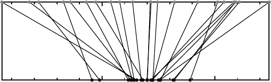
The model we have used also gives us updated estimates of the odds ratios of individual

studies, using the information that they all follow a Gaussian distribution. The idea, which is

Bayesian except that we replace the parameters ln(θ) and σ

with estimates from the data, is

outlined in Box 6.4. The result is shown in Figure 6.12. These updated estimates are called

COMMENTS AND FURTHER READING 169

0.50

ln(OR)

Figure 6.12 The estimated log-odds (upper row) and how they are shrunk (lower row) if we

assume the true log-odds come from a Gaussian distribution.

empirical Bayes estimates for the individual odds ratios, and the fact that we can strip the

estimates of some uncertainty this way is an example of a famous paradox pointed out by

Charles Stein (see Box 7.5). The paradox is that you can improve the estimate in one study

by using the estimates of other studies, which in this case is because we make the assumption

that the true log-odds follow a Gaussian distribution. This assumption provides a mechanism

for other studies to provide information on a single one.

One loose end remains: how do we get an estimate of σ

? Simple least squares does not

sufﬁce because of the way this parameter appears in the statistical model. The are different

ways we can estimate it, the simplest of which is to refer to the general maximum likelihood

theory. If we write down the log-likelihood of the problem above, we get a function of the

parameters θ and σ

, which we can maximize. This provides us with point estimates, and what

we have done above is use the point estimate of σ

from this as a true value in the description.

6.9 Comments and further reading

Most of the material here is very basic statistics, though the format is slightly unconventional.

Our main ambition has been to clarify the connection between the true CDF (the Platonic

world), and the world we observe, which consists of a limited amount of ﬁnite observed data,

summarized in the e-CDF. The e-CDF is my preferred substitute for histograms, which is

the way distributions usually are displayed. For discrete data histograms are not problematic,

describing frequencies as they do, but for continuous data one ﬁrst has to discretize the

data, and there is no unique way to do this. The precise way this is done may have a strong

inﬂuence on what the distribution looks like in a histogram. The main virtue of the e-CDF

is that it works for all kinds of distributions – continuous, discrete and mixed – which also

explains why the CDF is preferred over probability functions and probability densities in

this book. For an overview of the mathematical properties of the e-CDF, both exact and

large-sample theory, see Cs

aki (1984). Some key large-sample results are summarized

in Appendix 6.A.3.

When we introduced the t-test, we used the original data that William Gosset, publishing

under the pseudonym ‘Student’, used for illustration of his method. His test, now known as

Student’s (one-sample) t-test, was developed from a need to analyze small data sets accurately.

He could not use any of his own data for illustration (his employer, the beer company Guinness,

was afraid of disclosing company secrets), so he borrowed some medical data from Cushny

and Peebles, describing a crossover study on additional hours of sleep obtained when subjects