Kallen A. Understanding Biostatistics

Подождите немного. Документ загружается.

180 CORRELATION AND REGRESSION IN BIVARIATE DISTRIBUTIONS

The covariance is important for much the same reason the mean and variance are important;

it will be the key additional descriptor that deﬁnes the bivariate Gaussian distribution. The

factor that we integrate in the deﬁnition is positive when x and y are on the same side of

and m

, respectively, so the covariance will be positive if F (x, y) puts more weight in

those areas than in other areas. A positive covariance therefore implies that there is a net

covariation of X and Y , whereas a negative value implies that, on average, whenever one is

high, the other is low. It is a mathematical fact that C(X, Y )

≤ V (X)V (Y), and therefore

it is natural to describe the covariation of two stochastic variables in terms of the unit-free

correlation coefﬁcient

ρ(X, Y ) =

C(X, Y )

√

V (X)V (Y)

This correlation coefﬁcient ρ is by necessity a number between −1 and 1, and two

variables are said to be uncorrelated if ρ = 0. It is easy to show that two independent

variables are uncorrelated, but it is possible for dependent variables to be uncorrelated

(though not for Gaussian variables). As already mentioned, the correlation coefﬁcient is

a parameter that is heavily related to a bivariate Gaussian distribution, but it is not the

only way to describe correlation. Some alternative measures of correlation are outlined in

Box 7.1. To distinguish ρ from other correlation coefﬁcients, it is referred to as the Pearson

correlation coefﬁcient.

In passing we may note that if Z = (X, Y ) and m = (m

) we can deﬁne the matrix

V (Z) =



∞

−∞



∞

−∞

(z − m)(z − m)

dF (z), (7.1)

which will be a 2 ×2 matrix (z − m is a column vector in the integral) such that the diagonal

elements are the variances of the two components and the off-diagonal elements are the

covariance. We call this matrix the variance matrix of the bivariate stochastic variable. To

estimate it we use the corresponding discrete entity in which we replace the vector m with

the vector of arithmetic means ¯z, and the CDF with the corresponding e-CDF. The result is

the sample variance matrix

S =

n − 1



− ¯z)(z

− ¯z)

where the denominator is adjusted to make the corresponding variable unbiased. This has an

immediate generalization to higher-dimensional stochastic variables.

Example 7.1 Pearson’s correlation coefﬁcient is often used in medical statistics to describe

association, but when it comes to interpreting it, there is one salient point that is often missed.

Suppose that we have two outcomes (X, Y ) and we wish to understand the association between

them. Assume that their correlation coefﬁcient is ρ and let σ

and σ

denote their variances.

Each of the variables (X could be a biomarker, and Y a manifestation of a disease) is measured

with a measurement error. Assume that the measurement error for X has variance η

and that

for Y has variance η

. Let X



and Y



be the observed data. If measurement error is independent

of actual values, we have that C(X



) = C(X, Y ) = ρσ

, and therefore that the observed

BIVARIATE DISTRIBUTIONS AND CORRELATION 181

correlation coefﬁcient is

ρ(X



) =

ρσ



+ η



+ η



(1 + η

/σ

)(1 + η

/σ

)

If the measurement error is large relative to the variable variability, this means that the corre-

lation we observe gets attenuated. If we do not have precision in our measurements of X and

Y, the association may drown in the measurement noise.

We next wish to see how the Pearson correlation coefﬁcient relates to the odds ratio in the

simple case of a 2 ×2 table.

Example 7.2 Fora2× 2 table with cell probabilities p

, i, j = 1, 2, the covariance is easily

computed as p

− p

= p

− p

, so that Pearson’s correlation coefﬁcient is

given by

ρ =

− p

√

An estimate of this is called the phi coefﬁcient, and is obtained from cell counts as follows:

φ =

− x

√

To interpret ρ here, introduce δ by the relation p

= p

+ δ. Then we must also

have that p

= p

− δ, p

= p

− δ, and p

= p

+ δ, from which it

follows that δ = p

− p

. We obtain a relationship between δ and the odds ratio

θ = p

by inserting the expressions above to get

+ δ



+ p

1 − θ



+ p

= 0.

Solving this equation, we can express ρ = δ/

√

in the odds ratio θ and con-

stants that only depend on margins. This means that we can obtain a conﬁdence interval for ρ

conditional on the margins from a corresponding interval for the odds ratio. As example we

take the ﬁrst Hodgkin’s lymphoma example, for which the relation is illustrated in Figure 7.1.

The 90% conﬁdence interval (1.82, 4.71) for the odds ratio translates into the 90% conﬁdence

interval (0.15, 0.37) for ρ.

A related measure of association is Cohen’s κ, which is discussed in Box 7.2.

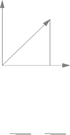
Figure 7.2 describes a geometric interpretation of the Pearson correlation coefﬁcient.

It shows how, given two independent and standardized stochastic variables, we can ﬁnd a

linear transformation of these which has correlation ρ to one of them. For future reference,

we note that the bivariate distribution F(y, z) = P(Y ≤ y, Z ≤ z)of(Y, Z ) in Figure 7.2 is

computed from



−∞

P(Y ≤ y|Z = ζ)dF

(ζ) =



−∞



X ≤

y − (sin θ)ζ

cos θ

|Z = ζ



(ζ),

182 CORRELATION AND REGRESSION IN BIVARIATE DISTRIBUTIONS

Box 7.2 Rater agreement and Cohen’s κ

Suppose that two pathologists independently examine a set of n slides for the pres-

ence or absence of a cell abnormality. One way to express the agreement between the

two (as an indicator of the reproducibility or interchangeability of their classiﬁcations)

is in terms of Cohen’s κ (kappa). To deﬁne this, arrange the possible outcomes in a

2 ×2 table so that the rows and columns are the classiﬁcations of the two patholo-

gists. If p

is the probability of a slide falling into cell (i, j ), the actual probability

of agreement is p

= p

+ p

and the probability of agreement by chance alone is

= p

+ p

. Cohen’s measure of agreement is now the excess probability

of agreement beyond chance,

κ =

− p

1 − p

To estimate this, we insert the observed cell counts into the expression for κ to get

ˆκ =

2(x

− x

)

+ x

We see that κ is proportional to the Pearson correlation coefﬁcient discussed in

Example 7.2 with a proportionality constant that only depends on margins. This means

that we can use the discussion in that example to transform a conﬁdence interval for

the odds ratio to one for κ. The result will be conditional upon margins, as for Fisher’s

exact test.

which means that

F (y, z) =



−∞



y − ρζ



1 − ρ



(ζ). (7.2)

−0.4

−0.2

0.2

0.4

0.6

Pearson correlation (ρ)

−1

Odds ratio (θ )

Figure 7.1 The connection between the odds ratio and the Pearson correlation coefﬁcient

in a (particular) 2 ×2 table with given margins.

ON BASELINE CORRECTIONS AND OTHER COVARIATES 183

Figure 7.2 From two independent stochastic standardized (mean zero and variance one)

variables X and Z we can construct a new standardized variable Y which has correlation ρ

with Z by rotation an angle θ such that ρ = sin θ. This is easily checked from the fact that

Y = (cos θ)X + (sin θ)Z. The correlation with X is cos θ.

For a continuous distribution this means that the bivariate density is given by

f (y, z) =



1 − ρ



y − ρz



1 − ρ



(z)

This formula will be used to derive the bivariate Gaussian distribution below.

The description of a general bivariate distribution in terms of parameters is more compli-

cated than in the univariate case. Percentiles, which should be the points deﬁning the same

height for the bivariate CDF, corresponds not to points on a line, but to curves in the plane.

This makes them not only hard to estimate, but also impossible to describe, except in a graph-

ical form. Therefore, to describe the location of a bivariate distribution the mean (vector)

becomes even more important than it was for univariate distributions, and multivariate Gaus-

sian distributions are even more important in multivariate statistics than univariate Gaussian

distributions are in univariate statistics.

7.3 On baseline corrections and other covariates

In this section we address the question how we best can utilize information on one variable in

the analysis of another when they are dependent. The setting will be the analysis of a clinical

trial, for which there is a choice between designing it as a parallel group study and a crossover

study. Sometimes there is no such choice, as when a long treatment period is needed, or the

effect of the drug is long-lasting, but when there is a choice, we need to understand the pros

and cons of the two designs. Some aspects of this are statistical and will now be discussed.

The setting is that we want to compare two treatments, an active drug and a matching

placebo, utilizing a particular outcome variable which we do not need to specify. Deﬁne the

following two stochastic variables:

•

X is the value of the outcome variable when the patient is given placebo;

•

Y is the value of the outcome variable when the patient is given the active drug.

184 CORRELATION AND REGRESSION IN BIVARIATE DISTRIBUTIONS

In theory both of these have a value for each individual, though we may only measure one of

them. Assume that (X, Y ) has a bivariate distribution with mean (m

), variances (σ

,σ

)

and (the Pearson) correlation coefﬁcient ρ. If we run a parallel group study, we will observe X

for some patients and Y for others, whereas if we run a crossover study we essentially observe

both, though not necessarily under identical conditions (which has consequences which will

be the subject of Section 8.7).

Our objective is to estimate the treatment difference  = m

− m

, which in the case of

a parallel group study is the mean difference between the groups. We wish to know which

design has the smallest standard error σ (the standard error is the standard deviation of the

estimator of ). Recall that it is /σ that deﬁnes the power of the study, so this determines

which design is the most efﬁcient when it comes to demonstrating effects.

If we assume that for the parallel group study each group contains n subjects, we have

that the variance of the observed mean difference is

V (

Y −

X) =

(σ

+ σ

whereas for the crossover study with n subjects it is

V (

Y −

X) =

(σ

+ σ

− 2ρσ

If we denote the estimator in the parallel group study by



and the estimator in the crossover

study by



, this means that we have the following relationship between their variances:

V (



) = V (



) − 2ρσ

/n.

If there is a positive correlation between the variables X and Y , which is to be expected in

this context, a two-period crossover study with n subjects is therefore always more efﬁcient

than a parallel group study with 2n subjects in total. These two study types can be considered

equivalent, since they involve the same number of assessments. In the extreme case of ρ = 0

they are equivalent from a statistical (though probably not from a cost) perspective, since this

condition implies that it does not matter if we reuse subjects in the study.

Conceptually things become clearer if we assume that the variance is the same for

X and Y and equal to σ

. In such a case we have that V (



) = 2σ

/n and that

V (



) = 2(1 − ρ)σ

/n. Split σ

into a sum σ

= σ

+ σ

, with σ

= ρσ

and

= (1 − ρ)σ

We can think of X − m

and Y − m

as constructed from a common stochastic variable Z

which has variance σ

, to which we have added a measurement error ξ, which has variance σ

The values of ξ are different and independent for the two measurements as well as independent

of Z. Under this assumption X and Y will have the same variance σ

+ σ

, whereas the

difference Y − X will have the same variance as the difference of two independent ξs, which

is 2σ

. We call σ

the between-subject variance, and σ

the within-subject variance. In this

notation we have that ρ = σ

/(σ

+ σ

) and the variance of



will be proportional to

+ σ

, whereas that of



will be proportional to σ

. In both cases the proportionality

factor is 2/n.

A more detailed modeling along these lines would suggest that we should write X as

above but that for Y, which is obtained on drug treatment, we should have the decomposition

Y = m

+ Z + τ + ξ, with the same Z as before but now adding not only an observational

error ξ but also a true treatment effect size τ which varies between subjects (and is independent

ON BASELINE CORRECTIONS AND OTHER COVARIATES 185

of the other components) with a variance σ

. This assumption implies that V (Y ) = V (X) +σ

so we expect the variance in the drug-treated group to be larger than in the placebo group.

In statistical modeling it is common practice to assume σ

= 0, which corresponds to a ﬁxed

treatment effect for all subjects. If we perform a t-test in such a situation, the estimated

(common) variance will be a compromise between σ

and σ

+ σ

. To avoid making this

assumption, and to allow for heterogeneity in the response to treatment, we need to replace

the classical ﬁxed effects models with mixed effects models.

One way to improve the efﬁciency of a (randomized) parallel group study would be to

measure the outcome variable not only at the end of treatment, but also at randomization,

providing a baseline measurement. We can then study the change from baseline as a new

outcome variable. The question is whether this helps. To see if it does, assume that the pair

(X, Y ) above consist of (baseline, end-of-treatment) measurements. The previous discussion

shows that

V (Y ) = σ

,V(Y − X) = σ

+ σ

− 2ρσ

from which it follows that V (Y − X) <V(Y ) precisely when ρ>σ

/2σ

. It is therefore

the correlation that determines whether we gain anything from looking at the change from

baseline or not. The cut-off point for this is a correlation of 0.5 when σ

= σ

, in which

case we can write the variances as V (Y ) = σ

+ σ

and V (Y − X) = 2σ

. Another way to

express the criterion that V (Y ) >V(Y − X) is therefore that the within-subject variability is

smaller than the between-subject variability. There is, however, a better way to approach the

problem, but before we discuss this, we need to understand why, and when, we can replace

the end-of-treatment value with the change from baseline and still get a valid estimate of .

Call the two groups A and B, and let superscript denote group membership, while

subscripts denote which variable we compute the mean of. It is a basic property of the

mean that

 = m

− m

= (m

Y−X

− m

Y−X

) + (m

− m

because the mean of a difference is the difference of the means. The ﬁrst parenthesis on the

right is what we measure when we analyze the change from baseline. This will estimate 

if and only if the second parenthesis is zero. If this is not the case, the two analyses estimate

different things. One way to guarantee equality at baseline is to randomize the study.

The answer to the question whether to choose Y or Y − X as outcome variable is that

we should choose neither. To see why, ﬁrst replace the change from baseline with the more

general variable Y − bX for some arbitrary constant b. If the groups have equal distribu-

tions at baseline, this variable also estimates , irrespective of our choice of b. To get the

most efﬁcient outcome variable we should therefore use Y − bX instead, where b is chosen

to minimize

V (Y − bX) = σ

+ b

− 2bρσ

This is a quadratic function in b, which has its minimum when b = ρσ

/σ

. This may appear

difﬁcult to apply in practice, since it looks like we need to have a good knowledge of the

distributional parameters in order to be able to compute b, but we will see that this is what is

done in an analysis of covariance.

The obvious next question is why we should content ourselves with taking a linear pre-

dictor for Y of the form bX – why not use some more general function of X?Ifwewant

186 CORRELATION AND REGRESSION IN BIVARIATE DISTRIBUTIONS

to predict Y from an observation x of X using a function g(x), how should we choose g(x)?

Suppose that we assess how good a particular prediction is by measuring the mean squared

error of the prediction E((Y − g(X))

); then the function g(x) that minimizes this is the

conditional expectation

g(x) = E(Y |X = x).

The importance of this function is obvious; by viewing X as an explanatory variable for Y ,

we can reduce the uncertainty about Y by observing X. The increase in precision is expressed

in the mathematical observation that

V (Y ) = E(V (Y|X)) + V (E(Y|X)).

In words: the total variance is the average of the conditional variances (essentially the unex-

plained variance) plus how much the predictor varies. We may also note that the overall mean

is the mean of all conditional means:

E(Y ) = E(E(Y |X)).

(This formula is sometimes called the tower formula for the mean.) The problem here is that we

may not know the exact bivariate distribution of (X, Y ), and therefore not be able to compute

the true predictor g(x). We may, however, know it up to some unknown parameters, so that we

have a family of functions g(θ, x) from which we want to pick one by obtaining an estimate

of θ from data. Alternatively, we can simply assume such a functional form, without having

any distributional knowledge to justify it. We then try to estimate θ from data by minimizing

the function Q(θ) = E((Y − g

(θ, X))

). This is the least squares method for the estimation of

parameters, the method Gauss used to ﬁnd Ceres. It will be the subject of Chapter 9.

The simplest choice for a function here, seen below to be appropriate for the bivariate

Gaussian distribution, is to use a linear function g(x) = a + b(x − m

), which is the best linear

predictor. As before m

is the mean of X. This case is what we considered above, and what

we have seen is that a = m

, the mean of Y, that b = C(X, Y )/V(X) = ρσ

/σ

, and that the

variance of the residuals is

V (Y − g(X)) = V (Y) − V (g(X)) = σ

(1 − ρ

This is what still remains to be explained in terms of other covariates.

7.4 Bivariate Gaussian distributions

The bivariate counterpart to a standardized Gaussian distribution N(0, 1) should have

= m

= 0 and σ

= σ

= 1, but there still are many of them, each corresponding to a

different degree of correlation between the components. One way to derive these distributions

uses equation (7.2) in its differentiated form, which shows that the density should be given by

(x, y; ρ) =



1 − ρ



y − ρx



1 − ρ



ϕ(x). (7.3)

BIVARIATE GAUSSIAN DISTRIBUTIONS 187

−3

−2

−1

−3 −2 −1 0 1 2 3

ρ =0

ρ =0.75

ρ =0 ρ =0.5 ρ =0.75

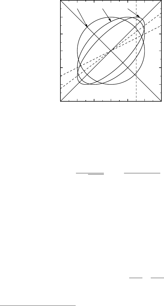
Figure 7.3 The shape of the height contours for standardized bivariate Gaussian distributions

for different correlation coefﬁcients.

Here ρ is the Pearson correlation coefﬁcient between the components. Writing out the expres-

sion and completing squares, we ﬁnd that this is

(x, y; ρ) =

2π



1 − ρ

exp



−

− 2ρxy + y

2(1 − ρ

)



. (7.4)

We denote this distribution by N

(0, 1,ρ) and its CDF by 

(x, y; ρ).

To describe the effect of ρ on the shape of the bivariate Gaussian distribution ge-

ometrically, look at Figure 7.3. It shows a contour

for the density function for three

different choices of the correlation coefﬁcient. Speciﬁcally, the curves are the ellipses

− 2ρxy + y

= 1 − ρ

for the choices ρ = 0, 0.5 and 0.75. (These are on the same

relative level, relative to the height of the density.) Note the oblique cross in the graph, which

corresponds to the two lines x = y and x =−y in the original coordinate system. For all

choices of ρ these lines represent the appropriate coordinate system in which to view data

(when ρ = 0 there is no preferred coordinate system). If we rewrite the equation for the

ellipse in this rotated coordinate system (45

◦

counterclockwise) with coordinates s, t, the

equation becomes

(1 − ρ)s

+ (1 +ρ)t

= 1 − ρ

⇔

1 + ρ

1 − ρ

= 1.

Functions of two variables can be graphically illustrated in the same way as nature topography is illustrated on

maps, by indicating height levels as curves in the plane.

188 CORRELATION AND REGRESSION IN BIVARIATE DISTRIBUTIONS

This expression conﬁrms what we can see in Figure 7.3, namely that if we increase ρ from

0 toward 1, the ellipse becomes more elongated in the x = y direction and narrower in the

x =−y direction. In other words, the closer the correlation is to one, the more concentrated the

distribution is around the line x = y. Similarly, if the correlation is close to −1, the distribution

is concentrated around the line x =−y.

On occasion we may have a 2 × 2 table in which both factors actually have continuous

distributions, but data collection has been dichotomized into yes/no categories only. We can

then analyze the table in such a way that we actually get a correlation measure between the

two factors. This is illustrated in the following example.

Example 7.3 The table below describes a cross-classiﬁcation according to whether or not a

group of workers were exposed to a particular environmental hazard, and whether or not they

showed symptoms of bronchitis:

Not exposed Exposed

Bronchitis 89 123

No bronchitis 453 318

Each of these two factors can be considered to vary in strength: there may be different degrees

of exposure and the bronchitis symptom may vary in severity. However, based on a cut-off

point for each, as in a medical test, each subject has found his place in this table. In this way

we may have a dichotomization of factors that are really continuous variables, but we have no

further recorded information on these. We therefore assume that the underlying continuous

data have a standardized bivariate Gaussian distribution, and that the table is obtained using

cut-offs a and b for exposure and bronchitis, respectively. As noted earlier, in order to ﬁt the

data to such a distribution we need to invoke the correlation coefﬁcient. In all there are three

parameters to ﬁt, and three conditions:

453/983 = 

(a, b; ρ), (89 + 453)/983 = (a), (453 + 318)/983 = (b).

The solution to this system is a = 0.129,b = 0.787,ρ = 0.241, where the last parameter is a

description of association. The correlation coefﬁcient in this hypothetical model is called the

tetrachoric correlation coefﬁcient.

The bivariate Gaussian is a distribution for which the best linear predictor is also the

best of all predictors. To see this, note that equation (7.3) implies that the conditional distri-

bution of Y given that X = x (whose density is ϕ

(x, y; ρ)/ϕ(x)) is also Gaussian, namely

N(ρx, 1 − ρ

). If we base our understanding of the bivariate Gaussian on the geometric de-

scription in Figure 7.3, it may be a little surprising to ﬁnd that the mean is ρx and not x, since

this graph shows that the distribution of the standardized bivariate normal (when ρ>0) is

concentrated along the line y = x. To see why the mean is ρx, look at the vertical dashed line

over the point x = 1.5 in Figure 7.3. It intersects the axes of the ellipse in an oblique manner

(actually 45

◦

), so more of it is below the line y = x than is above it. The mean is the mid-point

on this line within the ellipse, and the geometrically inclined reader can convince himself that

the line of means is precisely the line y = ρx.

REGRESSION TO THE MEAN 189

The general bivariate Gaussian distribution is deﬁned by the requirement that the mean

should be m = (m

) and its variance matrix should be  =





. This distribution

is denoted by N(m, ) and is deﬁned by the requirement that



X − m

Y − m



∈ N

(0, 1,ρ),

where ρ = σ

/σ

. For this distribution the discussion above shows that the distribution of

Y conditional on X = x is



+ ρ

(x − m

),σ

(1 − ρ

)



This implies that for a bivariate Gaussian distribution, the conditional mean of Y, given that

X = x, is the linear predictor

E(Y |X = x) = m

+ ρ

(x − m

). (7.5)

This last equation has some interesting consequences, which will be the subject of the

next section.

7.5 Regression to the mean

We will now use the fact that, for the bivariate Gaussian distribution, the best predictor is the

linear predictor, to illustrate an interesting and important point about the world and human

affairs. It is concerned with the situation where we make two consecutive observations of

something, and want to explain the effect we see by a causal relation. There is a speciﬁc

pattern to what happens in the long run, which leads to certain biases in causal explanations.

One example is found in sports, where being on the cover of a Sports Illustrated journal, or

being awarded the ‘Ballon d’Or’ in soccer, seems to imply poorer performance in the future.

Other examples include the following:

•

in education, where special treatment of poor performers all but guarantees their im-

provement;

•

in road safety policies, where actions taken at an accident-prone intersection almost

invariably have positive effects;

•

the observation that highly intelligent/successful parents often have less intelli-

gent/successful children.

The common denominator for all these examples is a law of nature called regression to

the mean, which was originally discovered by Francis Galton (see Box 7.3). He studied the

relationship between the height of a child and that of its parents. At his disposal he had human

data on the heights of 930 children and their 205 parents, which he sex-adjusted to ‘male’

heights by multiplying all women’s heights by 1.08. A quick summary of his result is that: