Kallen A. Understanding Biostatistics

Подождите немного. Документ загружается.

190 CORRELATION AND REGRESSION IN BIVARIATE DISTRIBUTIONS

Box 7.3 On Francis Galton, correlation and regression

The concepts of regression and correlation, as well as the bivariate Gaussian distribution,

were all introduced in the second part of the nineteenth century by an English polymath,

Sir Francis Galton.

Galton was nephew to Charles Darwin and was intrigued by The Origin of Species

and its identiﬁcation of the survival of the ﬁttest as the evolutionary force. Inspired

by this idea, Galton studied how talent ran in a number of families, including his own

and that of the Bernoulli (see Section 11.5). Based on this study Galton became in the

1860s a fervent advocate of positive eugenics, a term he coined in 1883, deﬁning it as

‘the study of all agencies under human control which can improve or impair the racial

quality of future generations’. (‘Positive’ refers to the fact that his suggested method

was to encourage marriage for the superior, instead of sterilizing the inferior as in the

US and some other countries.)

However, there was a disturbing pattern in the data, which was further clariﬁed in

a series of investigations into different sizes of seeds of the same species of sweet pea.

It had to do with two successive generations. When he ﬁnally had sorted it out and

published, he chose a different outcome variable, height in successive human genera-

tions, in order to drive home the message to a wider audience. This publication, which

also introduced the bivariate Gaussian distribution, had as its key message the notion

of regression to the mean: for standardized variables we have E(Y |X = x) = ρx,sowe

should on average expect some regression toward mediocrity. (Galton did not standard-

ize by mean and standard deviation, instead he used the median and half the interquartile

range.) This concept, regression, describes how the outcome of one variable predicts

the value of another.

What he did not note at the time was that the reverse is also true, that

E(X|Y = y) = ρy. The implication of this is that ρ is a more symmetric number related

to the two variables. It was not until later, when Galton worked in anthropology on

relations like that between a particular bone and the overall length of the body, that he

realized this symmetry and invented correlation, both the concept and the word, which

appeared in 1888 in a paper titled ‘Correlations and Their Measurement Chieﬂy from

Anthropometric Data’. Correlation is a spelling of the word ‘co-relation’ which was in

common use at the time.

•

when mid-parents (Galton’s term for the average parent height for each child) are taller

than mediocrity (Galton’s word for the median, which is the mean for the Gaussian

distribution), their children tend to be shorter than they are; and

•

when mid-parents are shorter than mediocrity, their children tend to be taller than

they are.

This summary is probably as good as any description of this phenomenon, in conjunction

with the tale in Box 7.4.

Galton’s observation is deduced from equation (7.5). To simplify the discussion, assume

that the marginal distribution of each generation is the same (same mean and variance). Then

E(Y |X = x) −m = ρ(x − m),

REGRESSION TO THE MEAN 191

Box 7.4 A tale about regression to the mean

Daniel Kahnemann is a psychologist who in 2002 received the Nobel prize in Economics

(actually, the Bank of Sweden Prize in honor of Alfred Nobel) for his work in behavioral

economics. In his speech of thanks he spoke about the following experience.

‘I had the most satisfying Eureka experience of my career while attempting to

teach ﬂight instructors that praise is more effective than punishment for promoting

skill-learning. When I had ﬁnished my enthusiastic speech, one of the most seasoned

instructors in the audience raised his hand and made his own short speech, which began

by conceding that positive reinforcement might be good for the birds, but went on to

deny that it was optimal for ﬂight cadets. He said,

“On many occasions I have praised ﬂight cadets for clean execution of some

aerobatic maneuver, and in general when they try it again, they do worse. On

the other hand, I have often screamed at cadets for bad execution, and in general

they do better the next time. So please don’t tell us that reinforcement works and

punishment does not, because the opposite is the case.”

This was a joyous moment, in which I understood an important truth about the world:

because we tend to reward others when they do well and punish them when they do

badly, and because there is regression to the mean, it is part of the human condition that

we are statistically punished for rewarding others and rewarded for punishing them. I

immediately arranged a demonstration in which each participant tossed two coins at

a target behind his back, without any feedback. We measured the distances from the

target and could see that those who had done best the ﬁrst time had mostly deteriorated

on their second try, and vice versa. But I knew that this demonstration would not undo

the effects of lifelong exposure to a perverse contingency.’

and, since −1 <ρ<1, this means that the expected difference from the mean for the son

(i.e., E(Y |X = x) −m) is smaller (closer to zero) than that for the mid-parent (i.e., x − m).

This is what Galton’s summary amounts to. The immediate consequence is that if we select

only parents with an above average mid-parent height, and look at their children, we will ﬁnd

that these are on average shorter than their parents. Still tall, but shorter. It works the other

way around also, in that if we look at tall children, their parents are expected to be, on average,

shorter than them, though still tall:

E(X|Y = y) −m = ρ(y − m).

Actually the son/father example is a better illustration of the special case than the mid-

parent/son example of Galton. This is because in Galton’s case the variances for X and Y are

not equal, and we therefore need to use the more general equation (7.5). Instead the mid-parent

height is an average of two heights, so we are probably closer to having σ

= σ

√

2 than

to having σ

= σ

. This means that the regression curve in this case is E(Y |X = x) −m =

√

2ρ(x − m), and it is only when ρ<1/

√

2 = 0.71 that we have regression to the mean (the

estimate for ρ in Galton’s data was 0.497).

Regression to the mean explains why we should avoid drawing conclusions about an

intervention from a change that has been observed over time. To expand on this, note that we

192 CORRELATION AND REGRESSION IN BIVARIATE DISTRIBUTIONS

can rewrite equation (7.5) as

E(Y |X = x) −x = m

− m

−



1 − ρ



(x − m

If we let this represent a situation with a pre-test and a post-test for which we assume a

common variance, and with an intervention in-between, the relation becomes

E(Y |X = x) −x =  − (1 − ρ)(x − m),

where m is the pre-test mean and  the true mean intervention effect. This expression gives

the apparent intervention effect, which is made up of two terms, the true intervention effect

 and a term which deﬁnes the regression to the mean effect. In a study this becomes a

statement about the bias in the expected value of the mean increase due to a difference to the

mean at baseline:

Y −

X = ¯x) =  − (1 − ρ)(¯x − m). (7.6)

We see that if we for some reason have ¯x<m, we will overestimate the effect, whereas the

reverse is true if ¯x>m. This observation becomes important when we compare two groups

and build our analysis on the change from baseline. In studies numerical differences at baseline

will lead to numerical differences at the end. We therefore need to build an analytic model

which adjusts for this, which is what is done in the analysis of covariance methodology (which

is actually an analysis of means) to be discussed in Section 8.8.

So far the discussion has been based on the assumption that the underlying distribution

is a bivariate Gaussian distribution. A natural question is to ask to what extent these obser-

vations hold true for other distributions. To investigate one particular extension, we build on

the decomposition

X = Z + ξ, Y = Z + η,

which is one way we can derive the bivariate Gaussian distribution from independent Gaus-

sian components, following the discussion on page 184. This assumption means that each

individual has a true value of the response variable, given by Z, but that value is measured

with (independent) errors on two occasions. Now drop the condition that Z has a Gaussian

distribution, but keep this assumption on ξ and η. Let g(x) denote the probability density for

the common marginal distribution of

X and Y. We can then compute the following expression

for the conditional mean (the derivation of which is outlined in Appendix 7.A.1):

E(Y |X = x) = x + σ

(ln g(x))



. (7.7)

This equation is also applicable in the related situation where we have a stochastic variable

(X = Z) distributed in a population, which we measure with an error (Y = Z + η), and we

wish to understand what we can say about the true value based on the observation. This is

related to an (in)famous observation in statistics, the Stein effect (see Box 7.5).

REGRESSION TO THE MEAN 193

Box 7.5 The Stein effect

Assume that there is a characteristic Z in a population which has a N(m, η

) distribu-

tion. When we measure Z, we do it with an error ξ which we assume has a N(0,σ

)

distribution, so that what we measure, X = Z + ξ, has a N(m, η

+ σ

) distribution.

Given that we have observed the measurement x in an individual, what can we say about

the true value for this individual? The regression to the mean equation shows that

E(Z|X = x) = m +



1 −

+ σ



(x − m),

which means that there is a shrinkage toward the mean, which is greater the larger σ

is relative to η

This observation is related to a famous result by Charles Stein from 1955. We do

not know m, but instead have a single observation x

(measured with error) on each

of n individuals. The intuitive answer to the question how we should estimate the true

value Z

for subject i, is that we should take Z

= x

. What Stein was able to prove, in

a more general context, was that we should really use an estimate

= ¯x + c(x

− ¯x)

for a constant c<1.

Comparing this with the observation in the ﬁrst paragraph, we see that we have re-

placed m with ¯x and that we should have something like c = 1 −σ

for the constant,

where s

is the sample variance of the observations. This is not quite true, but if we

redeﬁne s

by dividing by n − 3, instead of n − 1, it becomes so. This is done to ensure

unbiasedness, and was discussed in Box 6.4.

For the special case with the bivariate normal distribution, the σ

in equation (7.7)

is the within-subject σ

and g(x) = σ

−1

ϕ((x − m)/σ), where the new σ

is the total

variance, σ

= σ

+ σ

. In this case it follows that (ln g(x))



=−(x − m)/σ

,so

equation (7.7) becomes

E(Y |X = x) = x −

+ σ

(x − m) = x − (1 − ρ)(x − m).

We then rederive our regression to the mean equation.

What equation (7.7) tells us is that the correction term is increasing as long as g(x)is

increasing, and decreasing when g(x) is decreasing, which means regression toward the mode

of the density g(x), that is, the value x that deﬁnes the maximum of the function g(x) (a point

given by the solution to the equation g



(x) = 0). The mean, median and mode just happen to

be the same for the Gaussian distribution. However, this is only one particular model extension

of the bivariate Gaussian distribution.

Making statements about one outcome variable conditional on the observed values of

other variables is what we do when we consider the so-called linear models, which will be

the subject of Chapter 9. From a clinical trial perspective it is also important to understand

what it means to do something conditional on a condition of the type a<X<b. If we, as

before, consider X to be the baseline measurement of a clinical variable, a clinical protocol

in general deﬁnes a particular subpopulation of patients to study, which we hope will make

194 CORRELATION AND REGRESSION IN BIVARIATE DISTRIBUTIONS

Box 7.6 Conditioning in the bivariate Gaussian distribution

For a general (continuous) bivariate distribution, the conditional density of Y given a

condition such s a<X<b(a =−∞and b =∞are allowed), is given by

Y| a<X<b

(y) =



X,Y

(x, y)dx

P(a<X<b)

It follows that the expected value E(Y|a<X<b)isgivenby



∞

−∞



X,Y

(x, y)dxdy =



E(Y |X = x)dF

(x),

divided by F

(b) −F

(a). Note that

E(X|a<X<b) =



xdF

(x)/(F

(b) −F

(a)) = μ(a, b).

In the situation, discussed in the main text, where we observe a stochastic variable Z

twice with independent errors, equation (7.7) (what we denoted g(x) there is f

(x) here)

shows that

E(Y − X|a<X<b) =



(ln f

(x))



(x)dx

(b) −F

(a)

= σ

η(a, b), (7.8)

where η(a, b) = (f

(b) −f

(a))/(F

(b) −F

(a)), and also that

V (Y | a<X<b) = σ

(2 +σ

(λ(a, b) − η(a, b)

)),λ(a, b) =



(b) −f



(a)

(b) −F

(a)

it easier to demonstrate an effect. Such inclusion criteria will imply some kind of restriction

on the baseline measurements. For example, in asthma trials we may want to include only

patients who take a certain amount of rescue medication per day, and as outcome measurement

we may have a lung function measurement. We expect a symptomatic patient to have a

more compromised lung function than a non-symptomatic one, so the study population will

essentially be selected on a criterion of the form X ≤ a, though we have not speciﬁed a in the

protocol. How does regression to the mean manifest itself in such situations?

We consider again the bivariate Gaussian distribution for the case where the pre-treatment

and the post-treatment measurement have correlation ρ and the same variance σ

. We assume

that the population mean values are m and m + , respectively, for the two variables so that

the true treatment effect is . Our interest is in the estimation of this , which refers to the

whole population. Now assume that the net effect of the inclusion criteria is that we only

include subjects that fulﬁll the criterion a<X<bfor some a and b, possibly inﬁnitely small

or large, respectively. From the discussion in Box 7.6 we have that

E(Y − X | a<X<b) =  + (1 − ρ)σ

ϕ(

b−m

) − ϕ(

a−m

)

(

b−m

) − (

a−m

)

STATISTICAL ANALYSIS OF BIVARIATE GAUSSIAN DATA 195

The second term on the right shows the bias introduced in the estimate for the treatment effect

by having the inclusion criteria (assuming, of course, that our ultimate objective is to ﬁnd the

 in the whole population). There is no bias if ρ = 1 (which is obvious), and when a and b

are taken symmetrically around the mean m (because of the symmetry of ϕ(x)). Note that the

bias we get in the mean difference

Y −

X is not affected by sample size; it is determined by

the cut-off points alone.

Example 7.4 Assume that we work with an assay which, like all assays, measures with an

error. When measurements are (suspiciously) high, it may be tempting to reanalyze the same

sample and use the new measurement instead. What is the consequence of this? When the

true value in the sample is Z our ﬁrst measurement will be X = Z + ξ and the second will

be Y = Z + η, where ξ and η are independent measurement errors. Y is only observed when

X>a. The expected value for our measurement will be

E(X) + E(Y − X|X>a)(1 − F(a)) = E(X) − σ

g(a),

from which we see that we have a negative bias of size σ

g(a).

7.6 Statistical analysis of bivariate Gaussian data

We now wish to ﬁnd the two-variable analogue of the (univariate) t-test, which is about

obtaining (simultaneous) knowledge about (the components of) the mean vector in a bivariate

Gaussian distribution. The key observation is that for a variable Z with a bivariate Gaussian

distribution with mean m = (m

) and covariance matrix  =





, we have that

(Z − m)



−1

(Z − m) ∈ χ

(2).

Precisely as in the univariate case we usually do not know the variance matrix , and need

to estimate it with the sample variance matrix S. The theory that works in one dimension,

and was outlined in Appendix 6.A.1, can be generalized at the expense of some slightly more

complicated mathematics (see Appendix 7.A.2). The key information is that, for a sample

of size n,

n(n − 2)

2(n − 1)

(¯z − m)

−1

(¯z − m) ∈ F (2,n− 2).

This is a generalization of the univariate t-test and is called Hotelling’s T

-test. It is used to

obtain conﬁdence statements about the mean vector m by use of the conﬁdence function

C(m) = F

2,n−2



n(n − 2)

2(n − 1)

(¯z − m)

−1

(¯z − m)



, (7.9)

where F

a,b

(x) denotes the CDF of the F (a, b) distribution. This is a function of two variables,

which means that what was a conﬁdence interval for the univariate test now becomes a

conﬁdence region in the plane. The next example illustrates this.

196 CORRELATION AND REGRESSION IN BIVARIATE DISTRIBUTIONS

Mean of variable 2

−1 3210

0.8

0.9

0.95

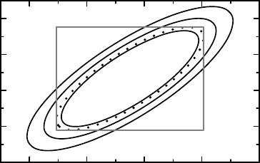
Figure 7.4 The solid contours deﬁne simultaneous conﬁdence regions for a Hotelling’s T

test. Also shown are the univariate conﬁdence intervals and the univariate conﬁdence region

as a dotted contour. See text for details.

Example 7.5 The Cushny and Peebles data mentioned in Example 6.5 consisted of 10 pairs of

data points, data which we assume come from a bivariate Gaussian distribution. Previously we

analyzed the mean difference of the two variables; now we wish to describe our conﬁdence in

the pairs of means. The mean vector is estimated as (0.75, 2.33), and the estimated covariance

matrix is



3.20 2.85

2.85 4.01



. Together these are all we need to calculate the conﬁdence function

in equation (7.9), which is described graphically by a contour plot in Figure 7.4. This graph

shows three contours of equal value for the function C(m), namely those corresponding to

the 0.8, 0.9 and 0.95 conﬁdence levels, respectively. The region enclosed by the last of these

levels corresponds to a conﬁdence region of (simultaneous) conﬁdence level 95% for the pair

of means. The corresponding univariate 95% conﬁdence intervals for the individual means are

indicated by the sides of the rectangle in the graph. This, however, does not enclose a region

with (simultaneous) conﬁdence level 95% for the mean vector, but by using the Bonferroni

correction we can show that the conﬁdence level is at least 90%.

Based on Figure 7.4 we can derive simultaneous conﬁdence limits for different combina-

tions of the two means. This means that we can compute as many functions as we wish without

losing credibility (in other words, no multiplicity correction is needed). Before we proceed,

however, look again at the conﬁdence function deﬁned by equation (7.9). It is computed by a

two-step procedure. First we compute the value of the quadratic form in the argument, from

which we derive the conﬁdence by applying a particular CDF to it. The choice F

2,n−2

(x)

as this CDF gives us simultaneous conﬁdence statements. If we want univariate statements,

that is, the limits of a single conﬁdence interval, we can use the F (1,n− 1) distribution

instead (which is the square of the t(n − 1) distribution). In other words, we use the

conﬁdence function

C(m) = F

1,n−1

((¯u − m)

−1

(¯u − m)). (7.10)

(Strictly speaking this may only hold true if the statement is based on a linear combination

of the components of m, as is the case below, because a linear combination of Gaussian

variables is a univariate Gaussian variable; see Appendix 7.A.3.) The 95% region obtained

STATISTICAL ANALYSIS OF BIVARIATE GAUSSIAN DATA 197

Mean of variable 2

−2 −1 43210

Mean of variable 1

0.8

0.95

0.995

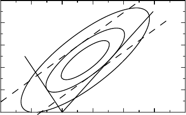
Figure 7.5 How to obtain univariate conﬁdence intervals for a mean difference and a mean

ratio from the bivariate conﬁdence function, deﬁned by the t distribution.

using this function is shown in Figure 7.4 as the dotted contour. It is the largest such contour

that ﬁts into the rectangle deﬁned by univariate conﬁdence intervals; the curve is tangent

to this rectangle at four points. The rectangle is therefore obtained by projecting the dotted

contour on to the respective axis.

Example 7.6 Continuing with the previous example, we now wish to derive univariate conﬁ-

dence intervals for two particular functions of the two means, using the (univariate) conﬁdence

function in equation (7.10). Three contours for this conﬁdence function, corresponding to the

conﬁdence levels 0.8, 0.95 and 0.995, respectively, are shown in Figure 7.5. The reason why

we choose these particular levels will soon become apparent.

We wish to identify the conﬁdence intervals both for the mean difference m

− m

and

for the mean ratio m

from this graph. To obtain the 95% conﬁdence interval for the mean

difference we consider the different lines m

− m

= θ, and identify those θ for which this

line is tangential to the 95% contour of C(m). These are indicated in the graph as the two

parallel dashed lines, corresponding to the two θ-values 0.70 and 2.46, respectively. These

two numbers are therefore the 95% conﬁdence limits for the mean difference, which agrees

with what we found in Example 6.5. Similarly, we obtain the conﬁdence limits for the ratio

by considering where the line m

= θm

is tangent to the 95% contour of C(m). These

two lines are illustrated in Figure 7.5 as solid straight lines, and the slopes of these provide

us with the limits −0.48 and 0.66, respectively, for the 95% conﬁdence interval.

There is also the contour for the level 0.995 shown in Figure 7.5. This is there to illustrate

a particular problem: the line corresponding to the lower conﬁdence limit for the ratio with

this conﬁdence level is horizontal, which means an inﬁnitely small lower conﬁdence limit. If

we require more conﬁdence than 0.995 we will therefore not get a ﬁnite interval. This will be

further explored below.

The intervals for the ratio of two means that we obtained above are called Fieller intervals

and are analytically described in Box 7.7. We see that two conditions need to be fulﬁlled in

order for this to provide ﬁnite intervals, and if we ask for enough conﬁdence, these conditions

will be violated for any data. In the next example we explore this further.

198 CORRELATION AND REGRESSION IN BIVARIATE DISTRIBUTIONS

Box 7.7 Fieller intervals for the ratio of means

Assume that we have a bivariate stochastic variable (X, Y ) with a Gaussian distribution

with mean (m

) and covariancematrix  = (σ

), and consider the ratio θ = m

We then have that

Y − θX ∈ N(0,σ

(θ)), where σ

(θ) = σ

− 2θσ

+ θ

If  is known, this means that the function

C(θ) = 



y − θx

σ(θ)



is a conﬁdence function for the ratio of the means. When we do not know  we may

estimate it with something that has a Wishart distribution, such as the sample variance, in

which case the estimate of σ

(θ) follows a χ

distribution, and we replace the Gaussian

CDF with the appropriate t distribution CDF.

There are conditions when such Fieller intervals (of conﬁdence level 1 − 2α)do

not produce ﬁnite intervals for the point estimate m

, conditions that occur for all

data if we ask for sufﬁciently high conﬁdence level (small α). The interval is deﬁned as

those θ for which we have that (y − θx)

≤ t

(θ), which can be rewritten as

− y

) − 2θ(t

− xy) +θ

− x

) ≥ 0.

The coefﬁcient on θ

has to be negative in order for this to deﬁne an interval, and the

condition for this is that |x|/

√

, which means that for the denominator m

there

is enough evidence that it is different from zero at the required conﬁdence level. The

other condition is that the discriminant is positive, which can be written



−1

z − t

) det >0,z=





The ﬁrst of these criteria is violated ﬁrst, and when it is, the interval will contain inﬁnity

since it allows for division by zero. When both criteria are violated, the inequality holds

true for all θ, because this case allows for the indeterminate number 0/0.

Example 7.7 The top part of the two-sided conﬁdence function for the mean ratio for the

Cushny and Peebles data is shown in Figure 7.6. The graph shows that the conﬁdence intervals

are somewhat ‘ﬁshy’ at very high conﬁdence levels. In fact, in order to have a ﬁnite interval

we must have a conﬁdence level less than 0.995. This level is shown as the lower dashed line

in the graph. It is the asymptote of the conﬁdence function in both inﬁnities. For a conﬁdence

level above this, but less than 0.9986, the conﬁdence region excludes a ﬁnite interval (and

includes inﬁnity), whereas for even higher conﬁdence levels all possible values constitute the

conﬁdence region; the data are insufﬁcient to provide any information about the parameter

with such high conﬁdence.

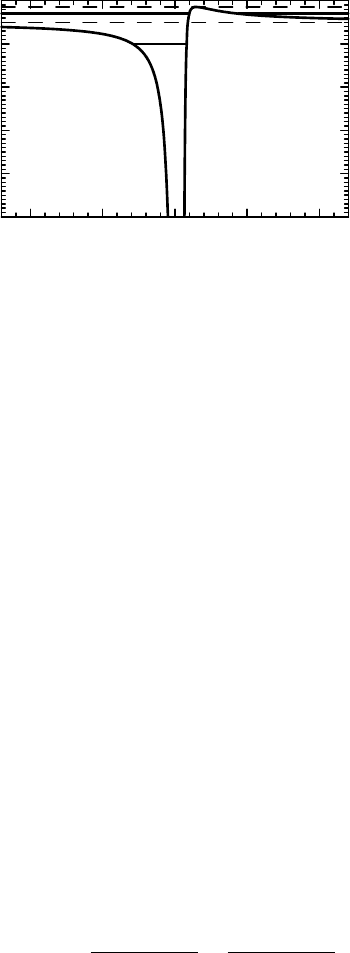
SIMULTANEOUS ANALYSIS OF TWO BINOMIAL PROPORTIONS 199

−10 − 10505

Mean ratio m

/ m

0.95

0.96

0.97

0.98

0.99

Conﬁdence in the ratio

Figure 7.6 The upper part of the two-sided conﬁdence function for the ratio of means for

the Cushny–Peebles data.

If instead we had drawn the one-sided conﬁdence function we would not have obtained

an increasing function from zero to one. Such a function cannot therefore work as a CDF,

which means that this is an example where we cannot interpret the conﬁdence function as a

distribution function, and which gave Fisher a headache with his ﬁducial concept.

7.7 Simultaneous analysis of two binomial proportions

The ﬁnal section of this chapter is rather mathematical in nature. It is about the general problem

of how we do inference on the parameters of interest in the presence of nuisance parameters.

The discussion to come, in the context of binomial parameters, is mainly explained in terms

of graphics, and it may be worthwhile for the less mathematically interested not to ignore it.

The ideas are the same as in the previous section.

In Chapter 5 we discussed how to compare binomial proportions from two different

groups. The assumption was that we have an observation x

from a Bin(n

) distribution,

and an observation x

from a Bin(n

) distribution which is independent of the ﬁrst. We

are interested in conﬁdence statements about various combinations of p

and p

.Inthe

discussion in Section 5.3 we noted that the approach taken there failed to take proper account

of all uncertainty in the data. Building on the ideas presented in the previous section, we will

now remedy this and obtain a simultaneous conﬁdence region for the pair (p

). Since it is a

simultaneous analysis, we can derive from this as many conﬁdence intervals for combinations

of p

and p

as we wish, without losing control of the overall signiﬁcance level. The starting

point for our investigation will be an observation we made in Section 5.4.1, namely that

C(p

) = χ



∗

− p

)

(1 − p

)

∗

− p

)

(1 − p

)



(7.11)

(where p

∗

is the estimate of p

) is an approximate conﬁdence function for p = (p

For illustration we again use the ﬁrst Hodgkin’s lymphoma data set, for which we

have p

∗

= 67/101 and p

∗

= 43/107. A few contours for the conﬁdence function C(p

)

are shown in Figure 7.7, the outermost of which is a 95% conﬁdence region for the

pair (p

). The other contours represent other conﬁdence levels. We will use the 95%