Kallen A. Understanding Biostatistics
Подождите немного. Документ загружается.


DIFFERENT WAYS TO DO LEAST SQUARES 251
Box 9.3 Why is analysis of means called analysis of variance?
The analysis of conditional means of an outcome variable on covariates when the rela-
tionship is a linear one (mathematically E(Y |X = x) = xθ), is called analysis of variance
if the covariates all are categorial (called factors), and it is called analysis of covariance
if at least one of the covariates is continuous and enters the model in such a way that
the mean is proportional (the slope) to its value. The reason why it is called an analysis
of variance in the former case is that the analysis consists of splitting sums of squares
into parts defining the estimation of factor effects, plus a final part of unexplained noise,
the residual sums of squares. Sums of squares estimate variances, which explains the
terminology. Such methods once led to convenient ways of doing the analysis by hand
when the data were balanced, but with present-day technology the matrix formulation
indicated in Box 9.2 is more powerful and easily implemented in computer software.
There is also a geometric formulation of the sums of squares approach, applicable
for all types of covariates, which allows a compact mathematical theory. In this
formulation data are considered to be part of a large Euclidean space, with a metric
defined by the covariance structure of the Gaussian model. Conditional means are then
orthogonal projections on subspaces representing different sub-models. By expressing
such spaces in matrix formulation, calculations with this approach are equivalent to the
matrix formulation.
We can also use this method if the variance structure is not constant, but depends on the
covariate(s). There is, however, an alternative and better way to approach this. In that method
we look for the θ that minimizes the weighted least squares
E
(Y − f (θ, X))
2
σ
2
(X)
.
An estimate of θ from data is obtained by minimizing the estimate of this expression:
Q(θ) =
1
n
n
i=1
σ(x
i
)
−2
(y
i
− f (θ, x
i
))
2
.
At this point we digress slightly to make a comment on the choice of weights. In certain
applications (modeling in pharmacokinetics is one), a least squares analysis is sometimes done
by weighting not on a conditional variance σ
2
(x
i
), but on either the value y
i
of the outcome
variable, or its square y
2
i
. Consider the latter case. Since ln x
2
− ln x
1
≈ x
−1
1
(x
2
− x
1
)we
have that
n
i=1
y
−2
i
(y
i
− f (θ, x
i
))
2
≈
n
i=1
(ln(y
i
) − ln(f (θ, x
i
)))
2
.
It is therefore more natural to do the actual estimation on a log scale instead in this case.
This may be because the original distribution resembles a lognormal rather than a normal
distribution. Similarly, a variance proportional to y
i
would mean that we should do the analysis

252 LEAST SQUARES, LINEAR MODELS AND BEYOND
on the square root of data instead of on the raw data. This is the case for Poisson data, for
which the square root transformation has a ‘normalizing’ effect. End of digression.
The notation above indicates that we know what the variance is as a function of the
covariates. In general this may not be true; there may be additional unknown parameters
φ in the variance, which we therefore write as σ
2
(x, φ). The standard ANOVA serves as an
example, where the variance is assumed constant but unknown, so that σ
2
(x, φ) = φ (which is
σ
2
). When φ enters as a proportionality factor like this, its value does not affect the estimation
of θ, but in other cases it will. However, we can never ignore φ altogether; it contributes to
the variance of the estimator, so when we want to describe our confidence in θ from data we
need to take it into account.
The situation is different if there is an overlap between θ and φ, which occurs, for example,
when the variance depends on the mean. This is the case for both binomial and Poisson data.
Since those parts of φ that are not in θ do not really play any role, we omit them from notation
and assume that the conditional variance of Y given that X = x is given by an expression
σ
2
(θ, x). The quadratic form Q(θ) then reads
Q(θ) =
1
n
n
i=1
σ(θ, x
i
)
−2
(y
i
− f (θ, x
i
))
2
.
This is a more complex situation to handle in full generality, because the derivative of Q(θ)is
not nearly as simple as before. If we differentiate Q(θ) we find that the derivative is the sum
of two terms, namely
U(θ) =
1
n
n
i=1
σ(θ, x
i
)
−2
f
(θ, x
i
)
t
(y
i
− f (θ, x
i
)) (9.1)
and a term involving the derivative of the variance. When the overriding purpose of the
analysis is to get a good fit of y to f (θ, x), it is tempting to replace the estimating equation
Q
(θ) = 0 with the equation U(θ) = 0. The solution to this equation is called the generalized
least squares (GLS) estimate. It is not as arbitrary as it may seem at first glance, because there
is a whole family of estimation problems for which this is the ‘right thing’ to do, which we
will discuss later in this chapter.
As an endnote to this, it is not difficult to obtain confidence statements about the GLS
estimate above, because the variance of the stochastic variable σ(θ, x)
−2
f
(θ, x)(Y − f (θ, x))
is
σ(θ, x)
−4
f
(θ, x)
t
V (Y |X = x)f
(θ, x) = σ(θ, x)
−2
f
(θ, x)
t
f
(θ, x),
where we have used the fact that V (Y|X = x) = σ
2
(θ, x). From this the variance of U(θ)
is easily derived, and we get the confidence function C(θ) = (U(θ)/
√
V (U(θ))), based on
large-sample theory.
9.4 Logistic regression, with variations
To illustrate the general discussion, we look at the example of accounting for covariates in
a model involving binomial distributions. We will do this with a view to estimating not prob-
abilities, but odds ratios. The definition of the odds ratio, OR = p
1
(1 − p
2
)/[p
2
(1 − p
1
)],
LOGISTIC REGRESSION, WITH VARIATIONS 253
Box 9.4 The logistic distribution
Logistic regression is associated with the logistic function
(x) =
1
1 + e
−x
,
which defines a distribution function with some interesting properties. One such property
is that it satisfies the logistic equation
(x) = (x)(1 − (x)). (9.2)
This equation is much used in ecology to describe a population that undergoes
exponential growth until it experiences crowding effects that limit its ultimate size
(here normalized to one) and is derived from the equation for exponential growth,
(x) = r(x), with a non-constant growth rate r = 1 −(x). It was introduced by
Verhulst in 1845, though the name came into general use 30 years later and is derived
from the French logistique, referring to the lodgement of troops.
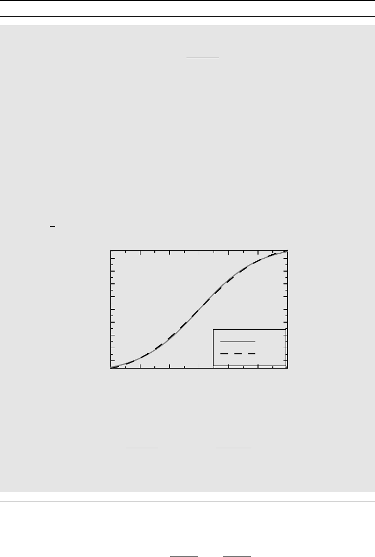
The logistic distribution closely resembles a Gaussian distribution, in fact, (x)
is almost indistinguishable from the Gaussian distribution (ax), where
a = 16
√
3/15π ≈ 0.59, as the following graph shows:
0.1
0.2
0.3
0.4
0.5
0.6
0.7
0.8
0.9
F (x)
−3 −2 −1 3210
x
Ψ(x)
Φ(ax)
The family of logistic distributions defined by
λ,γ
(x) = (−ln(λ) + γx) is closed
under the proportional odds model, because
θ
c
λ,γ
(x)
λ,γ
(x)
= θλe
−γx
=
c
θλ,γ
(x)
θλ,γ
(x)
.
This explains why we perform a logistic regression when we want to analyze odds
ratios.
means precisely that
ln OR = ln
p
1
1 − p
1
− ln
p
2
1 − p
2
.

254 LEAST SQUARES, LINEAR MODELS AND BEYOND
Introduce the notation
logit(p) = ln
p
1 − p
for the log-odds and let θ = ln OR be the log-odds ratio. What we have written above can
then also be written logit(p) = a + xθ, where x is +1 for group 1, and 0 for group 2, and a is
the log-odds for group 2 (we can also write it in other ways, for example with x taking values
±1 instead, which changes the meaning of the parameters a and θ but gives the same result if
we account for this change in meaning). This type of model is called a (linear) logistic model.
The general assumption is that the value of a binomial parameter p in a population depends
on observed covariate values x in such a way that logit(p) = xθ. The solution to this equation
can be written as p(θ, x) = h(xθ), where h(u) = 1/(1 + e
−u
) is called the logistic function
and is briefly presented in Box 9.4. The odds ratio θ is estimated by solving the GLS equation
U(θ) =
1
n
n
i=1
x
i
(y
i
− h(x
i
θ)) = 0.
The sum here is the difference between two sums. The first is
x
i
y
i
/n which is, since y
i
is
a 0/1 variable, the mean value of the covariate values for the records with y
i
= 1, times the
fraction of these among the total number of subjects. The second sum is the corresponding
predicted value from the model, since h(xθ) is the predicted probability of an event for a
record with covariate value x. The GLS equation therefore states that we wish to find the odds
ratio θ for which what we observe equals what we predict from the model using θ.
Example 9.2 In order to give an illustration of the logistic regression model we revisit the data
tabulated in Example 5.4. We have two dichotomous explanatory variables, the tonsillectomy
status and the study the data came from. An additive logistic regression model for these data
can be written
logit(p) = θ
1
+ θ
2
x
1
+ θ
3
x
2
,
where x
1
= 1 if the observation is on a (Hodgkin) patient and x
1
=−1 if it is on a control,
whereas x
2
= 1 if it is from Study 1 and x
2
=−1 if it is from Study 2. If we insert this into the
estimating equation and solve it, we find the parameter estimates θ
1
=−0.060,θ
2
= 0.192
and θ
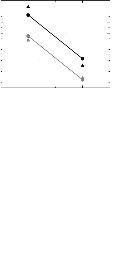
3
= 0.400. Figure 9.1 compares the predictions of the model, which are the (circle)
symbols connected with lines, with the corresponding empirical log-odds, which are the free-
floating (triangle) symbols. That the two lines are parallel is precisely what the model specifies
and the vertical distance between patients and controls defines the common logged odds ratio.
This means that the odds ratio is given by e
2θ
2
, from which we derive the estimate 2.22 with
95% confidence interval (1.73, 2.86). This is almost the same as the Mantel–Haenszel method
gave in Section 5.3.
We can also introduce an interaction term into the model. This means that we add one
more parameter θ
4
, such that
logit(p) = θ
1
+ θ
2
x
1
+ θ
3
x
2
+ θ
4
x
1
x
2
.
This extra parameter measures the interaction between studies and groups; it allows us to
adjust the two lines in Figure 9.1 so that they connect the observed log-odds (we say we
LOGISTIC REGRESSION, WITH VARIATIONS 255
−0.8
−0.6
−0.4
−0.2
0
0.2
0.4
0.6
0.8
log-odds
ControlsPatients
1Study
2Study
Figure 9.1 Data and model fit for a logistic regression for a meta-analysis of two studies on
Hodgkin’s lymphoma.
have a saturated model) and are no longer parallel. Testing the hypothesis θ
4
= 0 that there
is no interaction between study and patient group corresponds to the Breslow–Day test in
Section 5.5, and gives the same p-value. A little algebra shows that 4θ
4
is geometrically
the difference between the difference in the log-odds for patients and the difference for
the controls.
The results in the example are obtained assuming binomial distributions for data, but were
found to be very similar to what the Mantel–Haenszel approach gives, which is based on the
hypergeometric distribution, a conditional distribution for two independent binomials. This
conditional analysis is mainly used for case–control studies, since the meaningful parameter
is then the odds ratio. To expand on this, consider the situation where we have a case–control
study examining a particular exposure. We also have some additional confounders that we
want to adjust for in the analysis. Just as we can obtain Fisher’s exact test from a 2 ×2
table of two binomials by constructing a conditional test, we can derive a similar test for
this situation from the logistic regression model. To see how, we rederive the exact test in a
more general notation. A logistic regression model is defined by the probability function p(y)
defined by
i
n
i
y
i
e
y
i
(α+x
i
β)
(1 + e
(α+x
i
β)
)
n
i
= e
αy
+
+yxβ
i
n
i
y
i
(1 + e
(α+x
i
β)
)
n
i
, (9.3)
where yx =
i
y
i
x
i
as before. Here we have assumed that there are n
i
observations with
covariate vector x
i
and we have written the linear term as α + xβ in order to single out
the intercept α (x and β do not need to be univariate). The conditional distribution of Y on
the condition Y
+
= r eliminates α, but is somewhat involved from a notational perspective.
The key observation is that the probability for the event Y
+
= r is given by the sum of the
probabilities p(z) for all z such that z
+
= r, showing that the conditional distribution of Y

256 LEAST SQUARES, LINEAR MODELS AND BEYOND
given that Y
+
= r is given by
e
yxβ
i
n
i
y
i
{z;z
+
=r}
i
e
zxβ
n
i
z
i
.
In the special case where we have no additional covariates except exposure, and therefore
only one explanatory variable, with values 0 and 1, this probability function describes a
hypergeometric distribution.
Regression analysis of β using the general distribution above is referred to as conditional
logistic regression. To compute the estimating equation for β derived from this, using maxi-
mum likelihood, is rather computer-intensive, because we need to identify and calculate the
sum in the denominator. Once this is done, however, we can choose to proceed by appealing
to large-sample likelihood theory to derive approximate inference about β. Alternatively, we
can use combinatorial arguments.
However, this does not correspond to the Mantel–Haenszel test. We have used the variable
study as a covariate, whereas Mantel–Haenszel uses it to define a stratification. But we can
generalize to that situation too. Suppose that we want to assess the effect of an exposure in a
case–control study, and have at our disposal a series of strata, within each of which we have
a2×2 table with exposure-response numbers. The logistic regression model for this is
logit(p
i
) = α
i
+ xβ,
where p
i
is the probability for a case in stratum i and x a single 0/1 variable. In addition, we
have a series of stratum-specific intercepts. It is only β that is of interest here; all the α
i
are
nuisance parameters. When we compute the probability function for this case, we note that
each 2 × 2 table contributes two factors in the product formula in equation (9.3), one for each
of the two values of x. The probability function is therefore the following product over strata:
i
n
i1
y
i1
n
i2
y
i2
e
α
i
y
i+
+βy
i1
(1 + e
α
i
+β
)
n
i
.
To eliminate the α
i
we compute the conditional distribution on all the conditions y
i+
= r
i
corresponding to what we do for Fisher’s exact test for each individual table. With the same
argument as above, we find that the conditional distribution is
i
n
i1
y
i1
n
i2
r
i
−y
i1
e
βy
i1
k
n
i1
k
n
i2
r
i
−k
e
βk
,
which means (not surprisingly) that this is the product of a series of non-central
hypergeometric probabilities. The conditional logistic regression is therefore equivalent to
the Mantel–Haenszel method in terms of model; what differs slightly is the way the actual
parameter estimation is performed. To solve for β in the expression above, we consider the
logarithm of the probability function as a function of β and differentiate it, to obtain the
estimating equation
i
(y
i1
− E
β
(y
i1
)) = 0. In terms of estimation, the conditional logistic
regression approach in this case is therefore the same as the use of the Mantel–Haenszel
quadratic form Q
MH
(e
β
) in Section 5.5.
The logistic model is not the only possible model for binomial data. Instead of using the
logistic function as h(u) in the relation p(θ, x) = h(xθ) we can use other functions. The

THE TWO-STEP MODELING APPROACH 257
corresponding estimating equation becomes a weighted version of what constitutes the
estimating equation for the logistic model:
U(θ) =
n
i=1
w
i
(x
i
θ)x
i
(y
i
− h(x
i
θ)) = 0,w
i
(u) =
h
(u)
h(u)(1 − h(u))
. (9.4)
We have seen in Box 9.4 that the logistic function is almost indistinguishable from the func-
tion (au), where a = 0.59. To use the cumulative Gaussian as response function instead
is therefore an almost indistinguishable alternative, though the GLS equation becomes more
complicated. Such a model is called a probit model. Translating regression coefficients be-
tween the two models involves the use of the constant a.
There is one very good aspect of the probit model, compared to the logistic model. Suppose
that we have two binary outcomes, each of which we want to model with the linear model
a + bx, allowing for different regression coefficients for the two outcomes. Suppose further
that the two outcomes are correlated in some way. We can then simultaneously analyze the two
outcomes by replacing the univariate response function (u) with the bivariate standardized
Gaussian CDF
2
(u, v; ρ). If we organize the outcomes for each covariate value in a 2 × 2
table, we can model this in a way similar to what we did in Example 7.4.1 when we introduced
the tetrachoric correlation coefficient. The model in question is
p(1, 1|x) =
2
(a
1
+ b
1
x, a
2
+ b
2
x; ρ),
p(1, 0|x) = (a
1
+ b
1
x) −
2
(a
1
+ b
1
x, a
2
+ b
2
x; ρ),
p(0, 1|x) = (a
2
+ b
2
x) −
2
(a
1
+ b
1
x, a
2
+ b
2
x; ρ).
A similar extension does not come naturally for the logistic model.
Another useful response function for binomial data is h(u) = 1 − e
−e
u
. This is the func-
tion we should use when we are primarily interested in rates rather than proportions (see
Section 2.7). The logistic regression model is the appropriate model for the analysis of odds
ratios, but this model is the appropriate model to use when we analyze hazard rates, record-
ing only whether or not the event has occurred during the observation period. A regression
model for the hazard would then typically be of the form λ(x)T
i
= e
ln T
i
+xβ
, where T
i
is the
observation time for subject i. This means that the variable ln T
i
is part of the linear model,
but with a known coefficient, namely one. Such a variable is called an offset variable.
9.5 The two-step modeling approach
When we discussed the weighted least squares approach to estimation above we assumed that
the n observations in the data set were independent. We can, however, easily extend to the
case when the observations are dependent, as long as we account for the correlation between
the observations. This provides the building block for the two-step approach to modeling
that was indicated earlier and will revisited in the next chapter. The basic idea is that if the
observations y
i
are gathered into an n-vector y, f (θ) denotes the n-vector with components
previously denoted f (θ, x
i
) and V (θ) is the variance matrix of the outcome variable (possibly
dependent not only on θ, but also auxiliary parameters not included in the notation and
assumed known in the present discussion), then the GLS estimate of θ is obtained by solving

258 LEAST SQUARES, LINEAR MODELS AND BEYOND
the equation
f
(θ)
t
V (θ)
−1
(y − f (θ)) = 0.
To illustrate the two-step approach to analysis, suppose we have p groups and a p-vector
m = (m
1
,...,m
p
) of true group means, and assume that we have an estimator ˆm of m such
that ˆm ∈ N(m, ), where the variance matrix is known. That we may get correlations
when this is the output of a non-trivial first analysis is to be expected, but that should
be known is unrealistic. It is a convenient assumption for the moment, soon to be relaxed.
Next we impose a linear model on m, so that m = Bθ. This is not an equation with a unique
solution, because there are usually fewer parameters in θ than in m, so the design matrix
B has fewer columns than rows. The GLS equation (actually WLS in this case) for θ is
given by
B
t
−1
(ˆm − Bθ) = 0,
which is a linear system with solution
ˆ
θ = (B
t
−1
B)
−1
B
t
−1
ˆm ∈ N(θ, (B
t
−1
B)
−1
).
All this is a summary of some matrix algebra discussed earlier. What is different now is that
we will have the estimate of the m-vector as the result of a preliminary analysis, and what
we have just discussed constitutes a second step in the analysis. Why we want to do this may
be somewhat clarified if we revisit Example 9.2.
Example 9.3 In a two-step analysis of the data in Example 9.2 we first compute for each of
the four groups the (empirical) log-odds and its standard deviation (see Section 4.6.1). These
are shown in the following table (standard deviation in parenthesis; all correlations are zero
by design).
Patients, Study 1 Controls, Study 1 Patients, Study 2 Controls, Study 2
0.678 (0.211) 0.069 (0.152) −0.398 (0.197) −0.621 (0.097)
The standard errors are only estimates, but if we assume that they are exact, we can apply the
analysis discussed above. The model, which is illustrated by the straight lines in Figure 9.1,
is obtained if we apply the model m = θ
1
+ θ
2
x
1
+ θ
3
x
2
to the log-odds m. (As before, x
1
is
1 for patients and −1 for controls and x
2
takes value 1 for Study 1 and −1 for Study 2.) In
other words, putting the log-odds in a vector in the order of appearance in the table above, we
define the model m = Bθ, where
B =
⎛
⎜
⎜
⎜
⎝
11 1
1 −11
11−1
1 −1 −1
⎞
⎟
⎟
⎟
⎠
.
THE TWO-STEP MODELING APPROACH 259
It follows that the estimate of θ = (θ
1
,θ
2
,θ
3
)isgivenby
ˆ
θ = (B
t
−1
B)
−1
B
t
−1
⎛
⎜
⎜
⎜
⎝
0.678
0.069
−0.398
−0.621
⎞
⎟
⎟
⎟
⎠
=
⎛
⎜
⎝
−0.061
0.192
0.399
⎞
⎟
⎠
,
where is the diagonal matrix with the squared standard errors on the diagonal. We see
that the result is almost identical to what we found in Example 9.2. The slight difference
is explained by the difference between the we use here, which is the one obtained from
individual groups, and the corresponding used in the iterative process of the original model,
which is based on the model.
We may note in passing that if we add another column to B, consisting of zeros except
for the last element which is a one, and redo the analysis, we reproduce the saturated model
in Example 9.2. In this case this is an invertible transformation from the four group mean
log-odds to four new parameters, and for this case the variance matrix estimate is precisely
the same in the two analyses, and the results therefore identical.
In the first step of this example we reduced all data to estimates of a few parameters, accom-
panied by an estimate of the variance matrix for these estimates. This is what is summarized
in the table, and is a data reduction step. At this stage we could have taken the opportunity
to adjust the estimates for some covariates describing, for example, patient characteristics.
Whatever model we use in the first step, the second step is the same.
There may appear to be a price to pay when we do this analysis, since we need to use an
estimate of the variance of ˆm. However, the analysis is (almost) equivalent to the customary
analysis presented in Example 9.2, which also uses this approximation. It is not 100% correct,
but it is (almost) the standard large-sample approximation. But there are situations when we do
not even need to do it approximately. If our original data are from a linear model with Gaussian
data with a common variance σ
2
, then the analysis in Box 9.2 shows that ˆm ∈ N(m, σ
2
),
where = (A
t
A)
−1
is a known matrix derived from the design matrix A. This means that if
we use the estimate s
2
of σ
2
from the first model, we get an exact analysis, provided we use
the t distribution in the analysis (with the degrees of freedom from the first-step analysis).
Example 9.4 Suppose that we have an estimator ˆm which has a bivariate N
2
(m, ) distribu-
tion, and that we want to obtain information about m
2
, given that we know that m
1
= 0. This is
the ANCOVA problem, and it is an example of the analysis above. In fact, the model is m = Bθ
where B =
0
1
. The least squares estimate of θ is now given by
ˆ
θ = (B
t
−1
B)
−1
B
t
−1
ˆm.
The formula for the inverse of is
−1
= (det )
−1
22
−
12
−
12
11
,
which means that
(B
t
−1
B)
−1
= (det )/
11
=
22
−
2
12
/
11
=
2.1
.

260 LEAST SQUARES, LINEAR MODELS AND BEYOND
Inserting this in the formula above, we find that the estimate of θ is given by
ˆ
θ = ˆm
2
−
12
ˆm
1
/
11
. This is what we obtained in Section 8.8.
The two-step method is most useful in cases where there is a nonlinear relationship to be
described. From the discussion above we know that the equation to solve in order to estimate
θ for the model m = f (θ) is the GLS equation
f
(θ)
t
−1
(ˆm − f (θ)) = 0.
In order to obtain knowledge about θ we can either compute the variance of the stochastic
variable on the left here, or use the fact that the original assumptions mean that
Q(θ) = (ˆm − f (θ))
t
−1
(ˆm − f (θ)) ∈ χ
2
(p).
This gives us a confidence function to work with. As above, there are modifications in the
detail, depending on what information we have on . If we only have an estimate of
we need to modify the distribution appropriately, or appeal to large-sample theory and use
the estimated one as fixed to obtain reasonable approximations. Here ˆm has been presented
as adjusted means from a first-step analysis, but what it really consists of are estimates of
parameters from the model of this first analysis.
So far we have discussed how to get simultaneous confidence in all the model parameters.
What if we want a simultaneous confidence region for only a subset of these, with the remaining
ones considered nuisance parameters? More generally, what if we want a confidence interval
for a particular combination of the model parameters, and not a complex confidence region
for them all? This question was discussed, albeit in a special case, in Section 7.7, and a very
brief and superficial description of the method used, profiling, is as follows. Suppose we
want confidence information for a parameter η = g(θ).
1
Instead of minimizing Q(θ) to get an
estimate of θ, we then minimize it under constraints g(θ) = η for different η. This gives us a
function Q(η) of the new parameter alone, and we can obtain univariate confidence statements
about this by using the confidence function χ
1
(Q(η)). This is a general method that produces
reasonable results on most occasions, at least if the sample is not too small.
9.6 The effect of missing covariates
The classical ANOVA model and the logistic model, together with the other models for
binomial data discussed above, are members of a larger family of regression models, called
generalized linear models (GLMs). One common property of these is that the mean of
the outcome variable is modeled in terms of covariates, as an expression of the form
E(Y |X = x) = h(xβ), for some function h(u) called a response function. An important ques-
tion which then arises is the following. Suppose that there is a true model containing one set
of covariates, but that we have omitted to measure some of these and model the mean using
only the ones we have measured. What are the consequences? In the ANOVA situation we get
more unexplained residual variance, but no other effect on what we estimate. In the general
case, including the logistic model, the situation is more complicated.
1
This does not have to be one parameter; the function g(θ) can define more than one parameter, but it is simpler
if we think of it as a single parameter.